Random Graph Models with Non-Independent Edges Volume 2 - Issue 1

Zohre Ranjbar Mojaveri and Andras Farago*

• Department of Computer Science, The University of Texas at Dallas Richardson, USA

Received: November 24, 2020;   Published: November 30, 2020

*Corresponding author: Andras Farago, Department of Computer Science, The University of Texas at Dallas Richardson, USA

DOI: 10.32474/CTCSA.2020.02.000130

Abstract PDF

Abstract

Random graph models play an important role in describing networks with random structural features. The most classical model with the largest number of existing results is the Erd˝os-R´enyi random graph, in which the edges are chosen interdependently at random, with the same probability. In many real-life situations, however, the independence assumption is not realistic. We consider random graphs in which the edges are allowed to be dependent. In our model the edge dependence is quite general, we call it p-robust random graph. Our main result is that for any monotone graph property, the p-robust random graph has at least as high probability to have the property as an Erd˝os-R´enyi random graph with edge probability p. This is very useful, as it allows the adaptation of many results from Erd˝os-R´enyi random graphs to a non-independent setting, as lower bounds.
Random networks occur in many practical scenarios. Some examples are wireless ad-hoc networks, various social networks, the web graph describing the World Wide Web, and a multitude of others. Random graph models are often used to describe and analyze such networks. The oldest and most researched random graph model is the Erd˝os-R´enyi random graph G_{n, p}. This denotes a random graph on n nodes, such that each edge is added with probability p, and it is done independently for each edge. A large number of deep results are available about such random graphs, see expositions in the books [1-4]. Below we list some examples. They are asymptotic results, and for simplicity we ignore rounding issues (i.e., an asymptotic formula may provide a non-integer value for a parameter which is defined as integer for finite graphs).

The size of a maximum clique in G_{n, p} is asymptotically 2log_1/p n .

If G_{n, p} has average degree d, then its maximum independent set has asymptotic size (2n In d) / d .

The chromatic number of n, p G is asymptotically n/log_bn, where b=1-p

The size of a minimum dominating set in G_{n, p} is asymptotically n/log_bn, where b=1/1-p

The length of the longest cycle in G_{n, p}, when the graph has a constant average degree d, is asymptotically n(1− de^−d ) .

The diameter of G_{n, p} is asymptotically log n/ log(np), when np → ∞ . (If the graph is not connected, then the diameter is defined as the largest diameter of its connected components.)

If G_{n, p} has average degree d, then the number of nodes of degree k in the graph is asymptotically

However, the requirement that the edges are independent is often a severe restriction in modelling real-life networks. Therefore, numerous attempts have been made to develop models with various dependencies among the edges, see a survey in [2]. Here we consider a general form of edge dependency. We call a random graph with this type of dependency a p-robust random graph.

Definition 1 (p-robust random graph)

A random graph on n vertices is called p-robust, if every edge is present with probability at least p, regardless of the status (present or not) of other edges. Such a random graph is denoted by ~G_{n, p}.
Note that p-robustness does not imply independence. It allows that the existence probability of an edge may depend on other edges, possibly in a complicated way, it only requires that the probability never drops below p. Let us show some examples of p-robust random graphs.

1. First note that the classical Erd˝os-R´enyi random graph G_{n, p} is a special case of our model, since our model also allows taking all edges independently with probability p.

2. However, we can also allow (possibly messy) dependencies. For example, let P(e) denote the probability that a given edge e is present in the graph, and let us condition on k, the number of other edges in the whole graph. Let P_e(k) denote the probability that there are k edges in the graph, other than e. For any fixed k, set p(e | k) =1− (k +1) / n² ; let this be the probability that edge e exists, given that there are k other edges in the graph. Using that the total number of edges cannot be more than n(n −1) / 2 , we have that k ≤ n(n −1) / 2 −1 always holds. 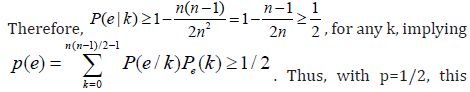random graph is p-robust. At the same time, the edges are not independent, since the probability that e is present depends on how many other edges are present.

3. For a given edge e, let r(e) denote the number of edges that are adjacent with e (not includinge itself). If e does not exist, then let r(e) = 0. Let the conditional probability that edge exists, 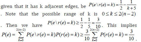Thus, with P = 3/10, this random graph is p-robust. At the same time, the edges are not independent, since the probability that e is present is influenced by the number of adjacent edges.

4. Consider the model described above in 3, but with the additional condition that each potential edge e has at least 3 adjacent edges, whether or not e is in the graph. What can we say about this conditional random graph? The same derivation as in 3, but with k ≥ 3, gives us that the new random graph will remain p-robust, but now with p = 3 / 8 .

If we have a random graph like the examples 2,3,4 above (and many possible others with dependent edges), then how can we estimate some parameter of the random graph, like the size of the maximum clique? We show that at least for so called monotone properties we can use the existing results about Erd˝os-R´enyi random graphs as lower bounds. Let Q be a set of graphs. We use it to represent a graph property: a graph G has property Q if and only if G∈Q . Therefore, we identify the property with Q. We are going to consider monotone graph properties, as defined below.

Definition 2 (Monotone Graph Property)

A graph property Q is called monotone, if it is closed with respect to adding new edges. That is, if G∈Q and G ⊆ G', then G'∈Q .

Note that many important graph properties are monotone. Examples: having a clique of size at least k, having a Hamiltonian circuit, having k disjoint spanning trees, having chromatic number at least k, having diameter at most k, having a dominating set of size at most k, having a matching of size at least k, and numerous others. In fact, almost all interesting graph properties have a monotone version. Our result is that for any monotone graph property, and for any n, p, it always holds that ~ G_{n, p}is more likely to have the property than G_{n, p} (or at least as likely). This is very useful, as it allows the application of the rich treasury of results on Erd˝os-R´enyi random graphs to the non-independent setting, as lower bounds on the probability of having a monotone property. Below we state and prove our general result.

Theorem 1 Let Q be any monotone graph property. Then the following holds:

Pr( G_{n, p}∈Q )≤ Pr( G_{n, p} ∈Q ) .

Proof: We are going to generate ~G_{n, p} as the union of two random graphs, G_{n, p} and G₂, both on the same vertex set V . G_{n, p} is the usual Erd˝os-R´enyi random graph, G₂ will be defined later. The union G_{n, p} U G₂ is meant with the understanding that if the same edge occurs in both graphs, then we merge them into a single edge. We plan to choose the edge probabilities in G₂, such that G_{n, p} U G₂ ~ ~G_{n, p}, where the “∼” relation between random graphs means that they have the same distribution, i.e., they are statistically indistinguishable. If this can be accomplished, then the claim will directly follow, since then a random graph distributed as ~G_{n, p} can be obtained by adding edges to G_{n, p} , which cannot destroy a monotone property, once G_{n, p} has it. This will imply the claim.

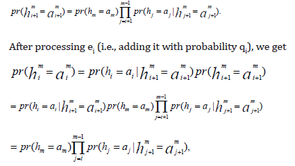
We introduce some notations. Let e₁, . . . , e_m denote the (potential) edges. For every i, let h_i be the indicator of the event that the edge e_i is included in ~ G_{n, p} . Further, let us use the abbreviation h_i^m = ( h_i,...,h_m ).For any a = ( a₁,...,a_m ) ∈ {0,1}^m, the event { h₁^m= a} means that ~ G_{n, p} takes a realization in which edge ei is included if and only a_i = 1. Similarly, {h_i^m = a_i^m} means { h_i=a_i,..,...,h_m = a_m } . We also use the abbreviation a_i^m =( _i,..., _m). Now let us generate the random graphs G_{n, p} and G₂, as follows.

Step 1: Let i = m.

Step 2: If i = m, then let q_m =Pr(h_m= 1). If i < m , then set q_i = Pr(h_i=1/h_i+1^m=a_i+1^m) where a_i+1^m indicates the already generated edges of G_{n, p} U G₂ .

Step 3: Compute 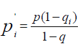.(1)

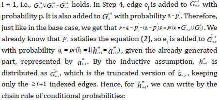
Step 4: Put ei into G_{n, p} with probability p, and put e_i into G₂ with probability 'q_i − p_i .

Step 5: If i > 1, then decrease i by one, and go to Step 2: else HALT.

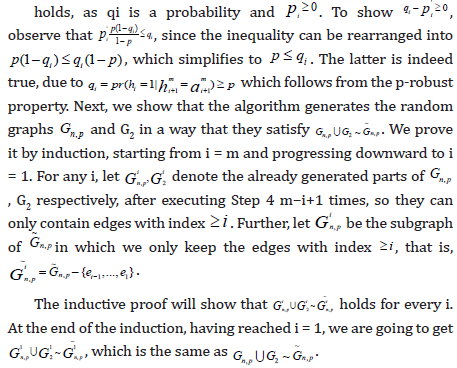
First note that the value q_i − p_i in Step 4 can indeed be used as a probability. Clearly, q_i − p_i≤ 1

Let us consider first the base case i = m. Then we have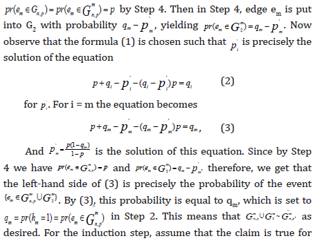

which, by the chain rule, is indeed the distribution of ~G_{n, p}ⁱting the induction.

Thus, at the end, a realization 1 {0,1} a = am∈ m of ~ Gn, p is generated with probability indeed creating ~G_{n, p} with its correct probability. Therefore, we get G_{n, p}UG₂~ G~_{n, p}arises by adding edges to G_{n, p} , which cannot destroy a monotone property. This implies the statement of the Theorem. As a sample application, we can claim that the random graph described in example 3, asymptotically has a maximum clique of size at least 2log_10/3 n , chromatic number at least n/ log_b n with b = 1/(1 − p) = 10/7, minimum dominating set at most log_b n/ , also with b = 10/7, and diameter at most . These follow from the known results about the Erd˝os-R´enyi random graph G_{n, p} , complemented with our Theorem. Note that such bounds would be very hard to prove directly from the definition of the edge dependent random graph model.

References

1. Bollobas B (2001) Random Graphs, Cambridge University Press, USA.
2. Farago A (2012) Network Topology Models for Multihop Wireless Networks. ISRN Communications and Networking 2012.
3. Frieze A, Karonski M (2016) Introduction to Random Graphs. Cambridge University Press, USA.
4. Janson S, Luczak T, Rucinski A (2000) Random Graphs, Wiley-Interscience.