


.png)

Lupine Publishers Group
Lupine Publishers
ISSN: 2637-6679
Research Article(ISSN: 2637-6679) 
Epidemic Prediction on Bionical Intelligent RGV Volume 5 - Issue 2
Received: March 19, 2020; Published: May 15, 2020
Corresponding author: Bin Zhao, School of Science, Hubei University of Technology, Wuhan, Hubei, China
DOI: 10.32474/RRHOAJ.2020.05.000209
Abstract
This paper studies the dynamic scheduling problem of bionical intelligent RGV, Modeling and Simulation of RGV scheduling problem in 4 cases of bionical intelligent machining system, and the simulation results of the model are tested by using three sets of real working data of RGV. Under known conditions, according to the working condition of a process, the RGV scheduling path is taken as the decision variable, and as much as possible clinker is processed as the objective function. Based on the idea of 0-1 planning, the RGV dynamic scheduling model is established when a process does not occur. Then a heuristic algorithm is constructed for the modeled model. Through simulation, the total production of materials under three sets of parameters is 383, 358, 392, and the system operation efficiency is not less than 98%. For the random failure of the processing system, the random failure probability is increased to 1% on the existing model, and the manual troubleshooting is performed. The duration is subject to the uniform distribution of 10~20 minutes, and the RGV dynamic scheduling model for single and double process machining under the condition of CNC probability failure is established. The total production of materials under one process is 357, 336, 362 respectively. The efficiency is as high as 98.3%, 95.9% and 98.4%; the total production of materials under the two processes is 223, 336, 362 respectively. Industry efficiency were 95.7%, 96.7% and 96.2%. Data simulation results show that the dynamic scheduling model for the establishment of RGV and practical algorithm.
Keywords: Multi-objective optimization; Bionical intelligent RGV; 0-1 planning; Optimal scheduling; Simulation
Introduction
The RGV is a bionical intelligent vehicle that can run freely
on a fixed track. The material processing system of RGV can save
huge labor costs for factories such as manufacturing factories and
logistics centers. Fig.1 gives an example of this guided-vehicle
system [1]. Unlike the classical material processing system, many
bionical intelligent RGVs in modern processing systems no longer
use fixed path, bionical intelligent R. The scheduling scheme of GV
is realized by programming [2,3]. Literature [4] presents several
algorithms for solving dynamic PDPTW model. RGV scheduling
problem is one of the most important issues in material processing
system [5,6]. The performance of material processing system has a
decisive impact on the efficiency of the whole equipment [7]. In the
design of scheduling path, the most common performance criterion
is to minimize the total distance [8,9] of RGV under given system
parameters. Due to the different working environments, there is still
no ideal algorithm to optimize the RGV scheduling path. Therefore,
there is still a lot of research space for the dynamic scheduling of
RGV in the specific system working environment (Figure 1).
The remainder of this paper is organized as follows. Section 2
describes the recent state-of-the-art in bionical intelligent vehicle’s
parameters. We discussion the condition of the problems in the
study we may meet in section 3. Section 4 is the hypothesis we
assumed in the study. And the section 5 is the symbol description.
Section 6 describes in detail the proposed dynamic programming
model based on 0-1planning. Section 7 tested the proposed method
using actual data. Finally, section 8 concludes this study, outlining
its contributions and possible directions for future work.
Figure 1: Guided-vehicle system schematic

Related Work
System operation parameters
The working environment studied in this paper consists of 8 CNCs, 1 RGVs, 1 RGV linear track, 1 feeding conveyor, 1 feeding conveyor and other equipment. Figure 2 shows the schematic diagram of this material processing system (Table 1). The operating parameters of this material processing system are derived from the latest available literature [10-13].
Figure 2:Intelligent processing system schematic

Table 1: 3 sets of data sheets for intelligent processing system operating parameters.

Three specific cases
1. The material processing operation of one process, the
same tool is installed for each CNC, and the material can be
processed on any CNC.
2. In the process of material processing in two processes, the
first and second processes of each material are processed by
two different CNCs in sequence.
3. The CNC may malfunction during the machining process
(the probability of failure is about 1%). It takes 10 to 20
minutes for each manual failure (unfinished material scrap)
[12-14]. After the troubleshooting, the CNC immediately joins
the sequence. Require separate consideration of material.
Processing operations for one process and two processes
Research task
1. We study the three working conditions and give the
dynamic scheduling model of RGV.
2. The model is tested by using three sets of data of the
system operating parameters in Table 1, and the scheduling
strategy of RGV and the operating efficiency of the system are
given.
Problem analysis
This paper studies the dynamic scheduling problem of RGV in intelligent processing system. According to the working requirements of RGV, under the actual operating rules of intelligent system, three general problems are considered: material processing operation in one process, material processing operation in two processes, and CNC failure. In the case of a process and two processes of material processing operations. The RGV dynamic scheduling model is established, and the corresponding algorithm is given. The practicality of the model and the effectiveness of the algorithm are tested by using the three sets of system operating parameter data respectively. The scheduling strategy of RGV and the operating efficiency of the system are given.
Analysis of task (1)
For the case (1): In the working process of the intelligent processing system, RGV can only load and unload one CNC at a time. The relationship between RGV and 8 CNCs per round can be expressed by 0-1 logic variable. The maximum amount of material obtained is taken as the objective function. The processing rule in the intelligent processing system is used as the constraint condition. Based on the 0-1 planning idea, the RGV dynamic scheduling model under a process processing demand is obtained. Construct a heuristic algorithm [15] and solve the model through simulation.
For the case (2): This paper considers that the maximum amount of RGV work is the largest as the objective function, and the constraint condition corresponding to the new machining rule is added to the original constraint to establish a double target based on the maximum number of materials obtained. The planned RGV dynamic programming model under the two-process processing requirements, and gives a concrete feasible solution algorithm.
For the case (3): When the CNC has a 1% probability of
failure, the repair time of the faulty CNC can be regarded as a
long processing time, and the time for manual troubleshooting is uniformly distributed within 10 to 20 minutes. After the fault is
removed, the CNC restarts. At this time, the waste material has been
removed, and the CNC immediately issued a demand instruction.
These work rules are embedded into the established dynamic
scheduling model to obtain the RGV dynamic programming model
under the condition of CNC probability failure, and the model is
solved by simulation.
The dynamic programming model is one of the optimization
methods in solving the dynamic scheduling problem [16,17]. The
problem it deals with is a multi-stage decision problem, which
starts from the initial state and reaches the end state by selecting
the intermediate stage decision [18,19]. These decisions form
a sequence of decisions and define an activity path (usually the
optimal route of activity [20]) that completes the entire process.
Initial state → │ decision 1 │ → │ decision 2 │ → ... → │ decision n │ → end state
The design of dynamic programming has a certain pattern, generally going through the following steps:
1. Division stage: According to the time or space characteristics of the problem, the problem is divided into several stages. These stages must be ordered or orderable (ie, no backwardness), otherwise the method fails.
2. Determining state and state variables: The various objective situations in which problems are developed into phases are represented in different states. Of course, the choice of state should be met without inefficiency. From the perspective of graph theory, if the state in this problem is defined as a vertex in the graph, the transition between the two states is defined as the edge, and the weight increment in the transfer process is defined as the weight of the edge, then the composition A directed acyclic weighted graph, therefore, this graph can be “topologically ordered [21]”, at least in the order of their topological ordering.
3. Determine the decision and write the state transition equation: Because decision and state transition have a natural connection, state transition is based on the state and decision of the previous phase to derive the state of this phase. So if the decision is determined, the state transition equation can be written. But in fact, it is often done in reverse, determining the decision based on the relationship between the states of the two adjacent segments. The sequence of decisions made at each stage is called a strategy.
4. Finding Boundary Conditions: The given state transition equation is a recursive equation that requires a recursive termination condition or boundary condition. The main difficulty of dynamic programming lies in the theoretical design. It is true that the role of dynamic programming is very large.
Analysis of task (2)
For task (2): Use three sets of system operation parameters to test the solution results, define WCNC (the working efficiency of the CNC), and use this index to measure the practicability of the scheduling model [21].
Problem Hypothesis
In order to reduce the complexity of the problem and simplify
the establishment and solution of the model, this paper makes the
following assumptions before establishing the model:
1. It is assumed that the CNC machining time is constant and
consistent for a certain process determined [22].
2. It is assumed that the RGV will not load or unload the RGV
until it moves to the CNC position after receiving the loading
request from the CNC [23].
3. It is assumed that the probability of failure occurs during
the processing of one process material and the processing of
materials in each step of the two processes is regarded as 1%.
4. Due to safety requirements, the tool cannot be replaced
in the middle until the system stops working after the system
is started.
5. Unless the system stops working for 8 hours of continuous
operation, the RGV’s movement, loading and unloading,
cleaning, etc. will not be stopped midway [24].
Symbol Description

Note: Other symbols are specified in the text.
Model Establishment
In the intelligent processing system, RGV can compare the
remaining machining time of 8 CNCs, the loading and unloading
time, and the time required for RGV to move to the corresponding
CNC position. This kind of RGV can judge the material order and
advance to the next round of optimal CNC [25]. Departure, making
the overall waiting time of 8 CNCs within 8 hours the least. In this
paper, RGV is used as the object of dynamic scheduling, and the RGV
dynamic scheduling model is established and solved. The optimal
scheduling scheme of RGV under three specific working conditions
is compared.
The intelligent working system has a continuous working time
of 8 hours, which makes 8 hours a complete processing process. The
goal of dynamic scheduling is to minimize the total non-working
time of the CNC within 8 hours. It is easy to know the total time of a
complete machining process of the intelligent processing system is
T = 8h = 28800s (1)
During a complete machining process, the machining system is started, the RGV executes the command from the initial position, and the machining is stopped near the 28800s, at which time the RGV returns to the initial position. The RGV workflow is shown in Figure 3.
Figure 3: RGV work flow chart

Model establishment of case (1)
For a processing system with only one process, the goal of the RGV dynamic scheduling model is to maximize the processing efficiency, that is, to process the material as much as possible within a given time, so that the number of processed materials is as large as possible. In the intelligent processing system, when one RGV is dispatched to load and unload 8 CNCs arranged on both sides, the k-th wheel of the RGV trolley can only go to and from the i-th CNC, and the 0-1 variable xi k is introduced.
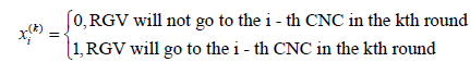 (2)
(2)In equation (2), i 1,2, n and in this context, eight CNCs in the
intelligent system are represented. When the material is in the
processing state, the corresponding CNC must be in the working
state.
When the material is in the non-processing state, the CNC
without the working state corresponds to it. Defining the RGV
operation for each CNC and only operating once and finally returning
to the starting position is a cycle. In the intelligent system, the RGV
goes to the i-th CNC to complete the working cycle of the working
cycle in the k-th round t1,i(k) can be expressed as
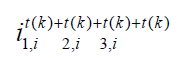 (3)
(3)Where t(k) is the time when the CNC is loaded and unloaded once, t2,i(k) is the time when the RGV 1, i2 ,i
completes the material cleaning, and t3,ki is the time when the RGV moves. When the CNC’s operating parameters are given, t1,i(k) t2,ki is known in the same operating system, so the relative size of the total time taken by the RGV to go to the i-th CNC to complete a working cycle when the RG is loaded in the k-th wheel is only determined. Through the above analysis, the objective function of the RGV scheduling model in one process is as follows
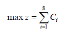 (4)
(4)Where Ci is the number of materials processed by the first CNC within 8 hours of a complete working process. Before the processing system is loaded, the CNC used is divided into two types: processed material and unprocessed material.
fi(k) (5)
)Where fi(k) is the material status on the first CNC before the k-th wheel is loaded. When the processing system is working, RGV can only work on one CNC at a time, loading and unloading, and the constraints on the decision variable xi(k) in the scheduling model are as follows
 (6)
(6)Within 8 hours of a complete machining process, the greater the total working length of 8 CNCs, the higher the efficiency of the processing system. We get
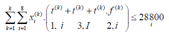 (7)
(7)Where k denotes the first loading of the processing system, i is
the CNC number in the system, and (7) means that the total working
length of 8 CNCs does not exceed 28800s during a complete
machining process.
After the processing system is turned on, the total working time
of 8 CNCs is 0 before the first round of loading. Which is
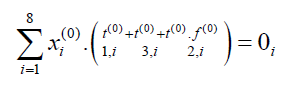 (8)
(8)In summary, after the simultaneous objective function and constraints, the RGV dynamic scheduling model with the largest total working time of 8 CNCs in 8h is established as follows
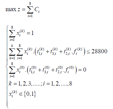 (9)
(9)Model establishment of case (2)
For the work with two processes, the first process and the second process of each material must be processed by two different CNC processes. For the entire two-step process, when a CNC completes the second process, the CNC is in a wait state and sends a demand signal to the RGV. When the RGV moves to the front of the CNC, the following steps are continuously performed:
Loading and unloading: Remove the clinker from this CNC; when the last time RGV was done in the process, put a new semiclinker into the CNC; when the last time RGV was done in the second step, the CNC did not put it in the CNC. Enter any material.
Cleaning operation: The clinker taken out is cleaned. At this
time, the position of RGV is unchanged in the orbit. RGV finds the next CNC to work according to the order of the demand signal and
the distance of the distance. Repeat the above steps of “loading and
unloading” and “cleaning operation” until the end of 8 hours.
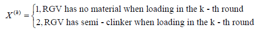
When the process requires two processes, the material
process status factor X (k) and the CNC process type factor Yi are
introduced. When the two factors match successfully, the RGV can
continue to load and unload. At this time, there are 256 kinds of
tool distribution schemes for 8 CNCs in the intelligent processing
system. This paper establishes a dual-objective planning model for
processing system RGV scheduling within 8 hours.
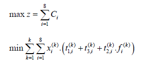
Based on the case (1) The objective function formula (4) with
the largest number of production materials within 8 hours has been
established, and the objective function is increased as follows
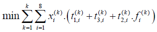 (10)
(10)Among them, the working parameters of the working system
such as the length of one loading and unloading t1,i(k) and the length
of one material cleaning t2,i(k) are given by Table 1.
For the work case with two processes, in addition to the
constraints (6)-(8), it is necessary to add and increase the
constraints as follows
 (11)
(11)Where equation (11) indicates that in a machining shift, a CNC can only process a specified process with one type of tool installed.
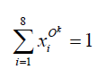
 (12)
(12)Where equation (12) represents the two states of the material to be processed. When loading in the k-th round, only when the material is successfully paired with the CNC can be loaded, which is
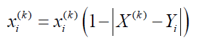 (13)
(13)In summary, in the case of two processes, the dual-objective planning model for RGV dynamic scheduling is as follows
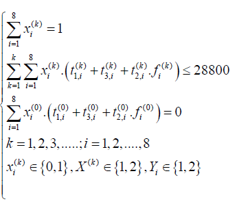 (14)
(14)Model establishment of case (3)
For the case of random failure in the intelligent processing
system, the situation (3) has pointed out that the probability
of failure is about 1%, and it takes 10 to 20 minutes to manually
process the failure. After the troubleshooting, the CNC immediately
joins the operation sequence. The RGV dynamic scheduling model
with random faults is established. On only one process and the
existing model with two processes, the constraints are added, so
that the improved scheduling model can collect fault information
and update the RGV work instructions.
During the working process of the processing system, the
probability of a CNC failure is determined, that is
 (15)
(15)Among them, it indicates that the i-th CNC has failed during the loading in the k-th round. After a failure, the manual repair time is 10 to 20 minutes, that is
 (16)
(16)Among them, Trepairk,i is the maintenance time after the failure of the i-th CNC in the k-th wheel loading. When Si k occurs, the i-th CNC at the time of loading in the k-th round cannot work normally according to the original setting, that is
 (17)
(17)At this point, manual repair is required to remove the waste, which is
 (18)
(18)In summary, the constraints (15)-(18) on the random failure in the processing system are added to the scheduling model (9) of a process, and the RGV scheduling model for one process and random failure is as follows
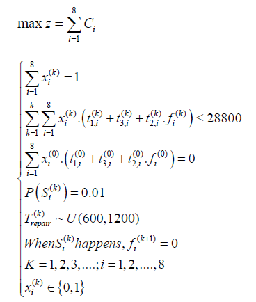 (19)
(19)Adding the constraints (15)-(18) on the random faults in the processing system to the scheduling model (14) of the two processes, the RGV scheduling model with two processes and random failures is as follows
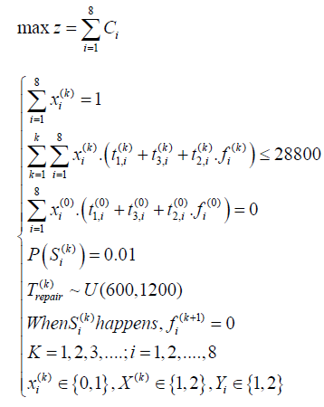 (20)
(20)Model Solution
The above-mentioned planning problems involve as many as tens of thousands of decision-making variables, and it is impossible to use traditional planning methods for computer solving. For the k-round machining process of 8 CNCs in RGV bionical intelligent processing system, the optimal candidate CNC is selected in real time, which involves the calculation of O N !. It is an NP problem, that is, the non-deterministic problem of polynomial complexity. Excellent solution. In this paper, a heuristic algorithm is constructed by each round of loading and unloading time, and the simulation problem model is used to solve such planning problems. Define WCNC (the system’s work efficiency), which is used to measure the efficiency of the RGV scheduling model under different types of work.
Solution of the model in three cases
For the case where there is only one machining program and no failure, use MATLAB to simulate the planning model (9). The results based on the three sets of given operating parameters are shown in Table 2. In Table 2, tup and tdown are the loading start time and the blanking start time, respectively. It can be found that when there is only one machining program and no failure occurs, the CNC is used to present a working cycle of 1 2 7 8. The RGV scheduling process at this time is shown in Figure 4. When RGV works in parameter group 1,383 materials are processed in one complete working process, which lasts 28758s; when RGV works in parameter group 2,358 materials are processed in one complete working process, which lasts 28795s; when RGV is parameter group 3 At work, a total of 392 materials were processed during a complete work, which lasted 28,709 s.
For the case of two machining programs without failure, use MATLAB to simulate the planning model (14). The results based on the three sets of given operating parameters are shown in Table 3-5. It can be seen from Table 3. that when the processing system with two processes works in parameter group 1, a maximum of 248 clinker can be produced in one complete work process, and CNCs numbered 1, 4, 6, and 8 are used in the first process. The CNC numbered 2, 3, 5, and 7 perform the second process on the material, and the total time is 28,710 s. The RGV scheduling process at this time is shown in Figure 5.
It can be seen from Table 4 that when the processing system with two processes works in parameter group 2, a maximum of 195 clinker can be produced in one complete working process, and CNCs numbered 1, 4, and 5 are used in the first process. The CNC numbered 2, 3, 6, 7 and 8 perform the second process on the material, and the total time consumption is 28945s. The RGV scheduling process at this time is shown in Figure 6. It can be seen from Table 5. that when the processing system with two processes works in parameter group 3, a maximum of 227 clinker can be produced in one complete working process, and CNCs numbered 2, 4, 6, 7 and 8 are used in the first process. The CNC numbered 1, 3, and 5 perform the second process on the material, and the total time consumption is 28818s. The RGV scheduling process at this time is shown in Figure 7. It is easy to know and has two processes and does not occur. In the randomly faulty RGV working system, among the three sets of given operating parameters, parameter group 1 can be used to produce the most clinker.
Figure 4: RGV Scheduling Diagram for case (1)

Figure 5: Case (2) Scheduling strategy for parameter group 1.

Figure 6: Case (2) Scheduling strategy for parameter group 2.

Figure 7: Case (2) Scheduling strategy for parameter group 3.

Table 2:Scheduling strategy for case (1).

Table 3:Case (2) Scheduling strategy for parameter group 1.

Table 4:Case (2) Scheduling strategy for parameter group 2.

Table 5: Case (2) Scheduling strategy for parameter group 3.

For the case of only one machining program and random failure,
use MATLAB to simulate the planning model (19). The solution
results based on the three sets of given operating parameters are
shown in Table 6.
In Table 6, when there are two machining programs and
there is a random failure, the CNC also exhibits of 357 complete
materials are processed in one complete working process, and 336
clinker materials are processed in the whole working process. The
random fault occurs once and lasts for 28810s. When RGV works
in parameter group 3, once A total of 362 complete materials were
processed during the complete work process, and random failures
occurred 4 times for a total duration of 28,780 s. For the case of two
machining programs with random faults, use MATLAB to simulate
the planning model (20). The results based on the three sets of
given operating parameters are shown in Table 7-9.
Table 6: Scheduling strategy with one operation and random failure.

Table 7: Scheduling strategy for parameter group 1 under two processes and random failures.

Table 8: Scheduling strategy for parameter group 2 under two processes and random failures.

Table 9: Scheduling strategy for parameter group 3 under two processes and random failures.

It can be seen from Table 7 that when the processing system
with two processes works in the parameter group 1, a maximum
of 248 clinker can be produced in one complete working process,
and the random failure occurs twice in each of the first and second
steps, numbered 1 The CNC of 4, 6, and 8 perform the first process,
and the remaining 4 CNCs perform the second process, with a total
time of 28,845s.
It can be seen from Table 8 that when the processing system
with two processes works in parameter group 2, up to 195 clinker
can be produced in one complete work process, and random failure
occurs once in process one, and does not appear in process two.
The total time is 28945s.
It can be seen from Table 9 that when the processing system
with two processes works in parameter group 3, up to 227 clinker
can be produced in one complete work process, and random failures
occur three times in process one and process two, respectively. It is
28818s. It is easy to know that for the RGV working system with
two processes and random failure of 1%, among the three sets of
given operating parameters, parameter group 3 can be used to
produce the most clinker.
Work efficiency solution
In an bionical intelligent system, RGV essentially provides services for the CNC, so that Tm is the total working time of a complete working process, n is the number of CNCs, tpi is the actual CNCs, and WCNC is the actual working time of the CNC in the entire working time, and defines the CNC. The work efficiency indicators are as follows
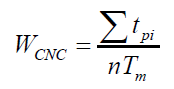 (21)
(21)where in equation (21), WCNC is the ratio of the sum of the actual working hours of all CNCs to the total working time of all CNCs, and the larger WCNC , the higher the operating efficiency of the bionical intelligent system. In the design of RGV dynamic scheduling, when the number of produced materials is as much as the objective function, the CNC waiting time should be reduced as much as possible, and the actual working time should be increased to improve the overall working efficiency of the bionical intelligent system. Using equation (21), the working efficiency of the machining system under three working conditions of one process, two processes and random failure is shown in Table 10 & 11.
Table 10: Work efficiency of situation (1) and situation (2).

Table 11: Working efficiency of one process and two processes under random failure.

In Table 10, Tm is the total working time of a complete working process, tpi is the number of CNCs, and WCNC is the actual working time of the CNC in the entire working time, which is obtained by equation (21). From Table 10, it can be seen that in a processing system with only one process and no random failure, RGV has the highest working efficiency when producing clinker according to the third group working parameters, and the processing system has two processes without random failure. Working with the first set of parameters is the most efficient
In Table 11, WCNC is also obtained by the formula (21). When the intelligent processing system has only one process but there is a random failure, RGV still produces the clinker according to the third group working parameters, and the working efficiency is the highest. When the processing system has two processes, but a random failure occurs, the work of the second group of parameters is performed. The most efficient. When using the established RGV scheduling model to plan the work of the intelligent processing system, no matter which operating parameters the processing system works, the processing efficiency of the system will not be lower than 95%.
Conclusion
In this paper, the dynamic scheduling of 8 CNC machining systems is studied. The RGV scheduling scheme under different working conditions is given, and the working efficiency of the system is calculated. The simulation results show that the dynamic scheduling model and algorithm for bionical intelligent RGV are feasible. In actual production, when the number of CNCs in the processing system increases, genetic algorithm and ant colony algorithm can also be considered to calculate the tool distribution scheme, thereby improving the calculation efficiency.
Conflict of Interest
We have no conflict of interests to disclose and the manuscript has been read and approved by all named authors.
Acknowledgement
This work was supported by the Philosophical and Social Sciences Research Project of Hubei Education Department (19Y049), and the Staring Research Foundation for the Ph.D. of Hubei University of Technology (BSQD2019054), Hubei Province, China.
References
- Le-Anh T, van der Meer J R, René B M de Koster (2004) Testing and classifying vehicle dispatching rules in three real-world settings. Journal of Operations Management 22(4): 369-386.
- Jünemann R, Schmidt T (2000) Materialflusssysteme: Systemtechnische Grundlagen. Springer
- Tompkins J A, White J A, Bozer Y A, et al. Facilities planning[M]. John Wiley & Sons, 2010.
- Savelsbergh M W P, Sol M (1995) The general pickup and delivery problem. Transportation science 29(1): 17-29.
- Luo J, Wu C, Hong W, Cheng Y, San-yao Xu, et al. (2010) Research on Scheduling of the RGV System Based on QPSO. IEEE ICCA 1169-1174.
- Le-Anh T, De Koster M B M (2006) A review of design and control of automated guided vehicle systems. European Journal of Operational Research 171(1): 1-23.
- Beamon B M (1998) Performance, reliability, and performability of material handling systems. International Journal of Production Research 36(2): 377-393.
- Gaskins R J, Tanchoco J M A (1987) Flow path design for automated guided vehicle systems. International Journal of Production Research 25(5): 667-676.
- Kaspi M, Tanchoco J M A (1990) Optimal flow path design of unidirectional AGV systems. The International Journal of Production Research 28(6): 1023-1030.
- Pei X, Liu T, Lu S, Liu Y, Pan W, et al. (2019) Study on Optimizing Dynamic Scheduling of Intelligent RGV[C]//3rd International Conference on Computer Engineering, Information Science & Application Technology (ICCIA 2019). Atlantis Press.
- Luo S (2019) RGV optimal scheduling scheme selection in multi-process scenario. AIP Conference Proceedings 2073(1): 020092.
- Yao Y (2019) Priority-based intelligent allocation scheduling model. AIP Conference Proceedings 2073(1): pp. 020100.
- Jia Y (2019) Based on Intelligent RGV Dynamic Scheduling Model of Particle Swarm Optimization. IOP Conference Series: Earth and Environmental Science IOP Publishing 252(5): 052135.
- Yin J Y, Chen N, Zhang Z T, Chen S S (2019) RGV Dynamic Scheduling Strategy Based on Network Cellular Automaton and Marko Model. IOP Conference Series: Materials Science and Engineering. IOP Publishing, 2019, 569(3): 032026.
- Meersmans P J M (2002) Optimization of container handling systems. 1-151.
- Bellman R, Kalaba R E (1966) Dynamic programming and modern control theory. New York: Academic Press 112.
- Liu Q, Dong M, Lv W, Chunming Ye (2019) Manufacturing system maintenance based on dynamic programming model with prognostics information. Journal of Intelligent Manufacturing 30(3): 1155-1173.
- Hubert L, Arabie P, Meulman J (2001) Combinatorial data analysis: Optimization by dynamic programming. SIAM 12: pp. 159.
- Bellman R E, Dreyfus S E. Applied dynamic programming[M]. Princeton university press, 2015.
- Bertsekas D P (1995) Dynamic programming and optimal control. Athena scientific 2: 1-153.
- Hansson T H, Oganesyan V, Sondhi S L (2004) Superconductors are topologically ordered. Annals of Physics 313(2): 497-538.
- Dai Y, Cao J (2019) Scheduler of CNC-RGV System based on STFF Model. 3rd International Conference on Computer Engineering, Information Science & Application Technology (ICCIA 2019). Atlantis Press
- Yin P (2019) Study on Optimal Scheduling of RGV in Industrial Production. IOP Conference Series: Materials Science and Engineering IOP Publishing 493(1):
- Li Y (2019) Scheduling analysis of intelligent machining system based on combined weights. IOP Conference Series: Materials Science and Engineering IOP Publishing 493(1): 012146.
- Yang F, Zhang H, Guo X, et al. (2019) Dynamic Schedule Strategy of RGV Based on the Weighted Directed Graph.


-

Mark E Smith
Bio chemistry
University of Texas Medical Branch, USA -

Lawrence A Presley
Department of Criminal Justice
Liberty University, USA -

Thomas W Miller
Department of Psychiatry
University of Kentucky, USA -

Gjumrakch Aliev
Department of Medicine
Gally International Biomedical Research & Consulting LLC, USA -

Christopher Bryant
Department of Urbanisation and Agricultural
Montreal university, USA -

Robert William Frare
Oral & Maxillofacial Pathology
New York University, USA -

Rudolph Modesto Navari
Gastroenterology and Hepatology
University of Alabama, UK -

Andrew Hague
Department of Medicine
Universities of Bradford, UK -

George Gregory Buttigieg
Maltese College of Obstetrics and Gynaecology, Europe -

Chen-Hsiung Yeh
Oncology
Circulogene Theranostics, England -
.png)
Emilio Bucio-Carrillo
Radiation Chemistry
National University of Mexico, USA -
.jpg)
Casey J Grenier
Analytical Chemistry
Wentworth Institute of Technology, USA -

Hany Atalah
Minimally Invasive Surgery
Mercer University school of Medicine, USA -

Abu-Hussein Muhamad
Pediatric Dentistry
University of Athens , Greece
