Prediction of TIG Process Parameters Needed to Eliminate Post Weld Crack Formation and Stabilize Heat Input in Mild Steel Weldment using Artificial Neural Network (ANN) Volume 4 - Issue 1

Pondi P, Achebo J and Ozigagun A*

• Department of Production Engineering, Faculty of Engineering, University of Benin, Nigeria

Received: March 25, 2021;   Published: April 07, 2021

*Corresponding author: Ozigagun A, Department of Production Engineering, Faculty of Engineering, University of Benin, P.M.B 1154, Benin City, Edo State, Nigeria

DOI: 10.32474/MAMS.2021.04.000179

Abstract PDF

Abstract

One of the limitations associated with response surface methodology (RSM) is that an understanding of the trend and pattern of the input variable is required for every model. It means therefore that the performance of RSM is dependent on the beauty of experimental design. Therefore, to predict the response variables beyond the scope of experimentation, predictive model such as artificial neural network (ANN) is required. The focus of the study is to apply artificial neural network for the prediction of tig process parameter such as Brinell hardness number (BHN), heat input (HI) and cooling rate (CR) which is required for eliminating post weld crack formation, and stabilizing heat input in mild steel weldment. The key input parameters considered in this work are welding current, welding voltage and welding speed while the response or measured parameters are Brinell hardness number (BHN), heat input (HI) and cooling rate (CR). Using the range and levels of the independent variables, statistical design of experiment (DOE) using central composite design (CCD) method was done. Hundred (100) pieces of mild steel coupons measuring 60 x 40 x10 were used for the experiments. The experiment was performed 20 times, using 5 specimens for each run. The plate samples were 60 mm long with a wall thickness of 10mm. The samples were cut longitudinally with a single-V joint preparation. The tungsten inert gas welding equipment was used to weld the plates after the edges have been bevelled and machined. The welding process uses a shielding gas to protect the weld specimen from atmospheric interaction. For the analysis of the measured variables artificial neural network was employed. To implement the neural network, a learning rate of 0.01, momentum coefficient of 0.1, target error of 0.01, analysis update interval of 500 and a maximum training cycle of 1000 epochs were used. The network generation process divides the input data into training data sets, validation and testing. For this study, 60% of the data was employed to perform the network training, 25% for validating the network while the remaining 15% was used to test the performance of the network.
From the result obtained, it was observed that the network performance was very good with performance errors of 3.4393e-05, 6.3500e-09 and 0.00034858 representing Brinell hardness number, heat input and cooling rate, respectively.

Keywords: Tig process parameters; Brinell hardness number (BHN); Heat input (HI); Cooling rate (CR); Artificial neural network (ANN)

Introduction

It is a well-known fact that most welders mainly focused on bead geometry and aesthetics of the weld structure, but the reduction in post weld cracks which determines the overall quality of weldment has not been paid much attention [1]. These problems can be solved with the development of mathematical models through effective and strategic planning, design, and execution of experiments [2]. Setiono et al. [3], reveals that neural networks (NNs) have been successfully applied to solve a variety of application problems including classification and function approximation. They are especially useful as function approximators because they do not require prior knowledge of the input data distribution and they have been shown to be universal approximators. [4], conducted a research on improving the corrosion-resistant properties of carbon steel using cladding process. The main problem faced in cladding is the selection of optimum combinations of process parameters for achieving quality clad and hence good clad bead geometry. The research highlights an experimental study to predict various input process parameters (welding current, welding speed, gun angle, contact tip-to-work distance, and pinch) to get optimum dilution in stainless steel cladding of low carbon structural steel plates using Gas Metal Arc Welding (GMAW). Experiments were conducted based on central composite rotatable design with full replication technique, and mathematical models were developed using multiple regression method. The developed models were checked for adequacy and significance. Using Artificial Neural Network (ANN) the parameters were predicted, and percentage of error was calculated between predicted and actual values [5].
Generally, all welding processes are used with the aim of obtaining a welded joint with the desired weld-bead parameters, excellent mechanical properties with minimum distortion [6,7]. To determine the welding input parameters that lead to the desired weld quality, application of Design of Experiment (DOE), evolutionary algorithms and computational network are widely used to develop a mathematical relationship between the welding process input parameters and the output variables of the weld joint. The research on parameter optimization of different types of welding for obtaining various responses in output have been done by several researchers using a wide range of materials. They make use of various types of methods, techniques, and mathematical models for evaluating and obtaining results.

Research Methodology

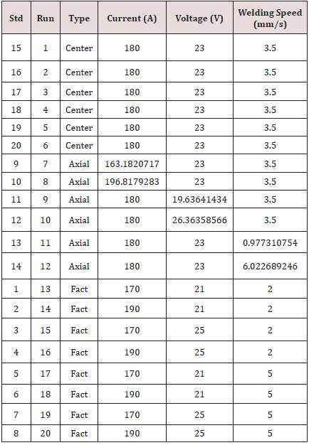
The key input parameters considered in this work are welding current, welding voltage and welding speed while the response or measured parameters includes Brinell hardness number (BHN), heat input (HI) and cooling rate (CR). The range and level of the experimental variables used for statistical design of experiment are presented in Table 1. Using the range and levels of the independent variables presented in Table 2, statistical design of experiment (DOE) using central composite design (CCD) method was done. The total number of experimental runs that can be generated using the CCD is defined as.

Where:
N is the number of experimental runs based on CCD design
2n is the number of factorial points
n0 is the number of center points
2n is the number of axial points
n is the number of variables

Using Equation 1, twenty (20) experimental runs were generated based on the central composite design method and presented in Table 2.

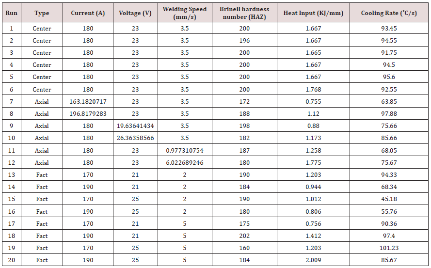
Applying the design of experiment presented in Table 2, 100 pieces of mild steel coupons measuring 60 x 40 x10 were used for the experiments. The experiment was performed 20 times, using 5 specimens for each run. The plate samples were 60 mm long with a wall thickness of 10mm. The samples were cut longitudinally with a single-V joint preparation. The tungsten inert gas welding equipment was used to weld the plates after the edges have been bevelled and machined. The welding process uses a shielding gas to protect the weld specimen from atmospheric interaction. For this study, 100% pure Argon gas was used. The weld samples were made from 10mm thickness of mild steel plate; the plate was cut to size with the power hacksaw. The edges grinded and surfaces polished with emery paper and the joints welded and thereafter, the responses were measured and recorded. The measured response corresponding to the input variable is presented in Table 3. For the analysis of the measured variable (Brinell hardness number, heat input and cooling rate), artificial neural network was employed. The step-by-step methodology of applying neural network is discussed as follows.

Generation of Input Data

Where. x_i; is the normalized value of the input and output data
x_min; and x_max are the minimum and maximum value of the input and output data
x is the input and output data.

Selection of training algorithm and hidden neurons

Input and output data training resulting in the design of network architecture is of paramount importance in the application of neural network to data modelling and prediction. To obtain the optimal network architecture that possess the most accurate understanding of the input and output data, two factors were considered. First was the selection of the most accurate training algorithm and secondly, the number of hidden neurons. Based on this consideration, different training algorithm and hidden neurons were selected and tested to determine the best training algorithm and accurate number of hidden neurons that will produce the most accurate network architecture. Selectivity was based on (r2 and MSE).

Network training/performance of MNN

To train the network, 3 runs of 1000 epochs, each were used. In addition, cross validation data representing about 15% of the total input data were introduced to monitor the progress of training and prevent the network from memorizing the input data instead of leaning which was a common problem associated with overtraining. The progress of the training was checked using the mean square error of regression (MSE) graph for training and cross validation

Network testing/validation

To test the efficiency of the trained network, 25% of the input data was introduced to the network.

Results and Discussion

To apply ANN for the prediction of Tig process parameters, two important factors were considered, and they include.
a. Selection of the most accurate training algorithm and
b. Determination of the exact number of hidden neurons
Based on this consideration, different training algorithm and hidden neurons were selected and tested in order to determine the best training algorithm and the exact number of hidden neurons that will produce the most accurate network architecture. Table 4 shows the different training algorithm that were tested and their performance. Based on the result of Table 4, improved second order method of gradient also known as Levenberg Marquardt Back Propagation training algorithm (LMBPTA) was selected as the best since it has the highest coefficient of determination (R2) and the lowest mean square error of regression (MSE). To determine the exact numbers of hidden neuron, different numbers of hidden neurons were tested to create a trained network using Levenberg Marquardt Back Propagation training algorithm. The number of hidden neurons corresponding to the lowest MSE and the highest R2 as presented in Table 5 was selected to design the network architecture.
Based on the results of Tables 4 & 5, Levenberg Marquardt Back Propagation training algorithm having 10 hidden neurons in the input layer and output layer was used to train a network of 3 input processing elements, namely, current, voltage and welding speed and 3 output processing element Brinell hardness number (BHN), heat input (HI) and cooling rate (CR). The input layer of the network uses the hyparbolic targent (tan-sigmoid) transfer function to calculate the layer output from the network input while the output layer uses the linear (purelin) transfer function. The number of hidden neuron was set at 10 neurons per layer and the network performance was monitored using the mean square error of regression (MSEREG). To characterize the network training function, Trainlm was employed. Trainlm is a network training function that updates weight and bias values according to Levenberg-Marquardt optimization. Although, it requires more memory than other supervised learning algorithm, Trainlm remains the fastest back propagation learning algorithm in MATLAB toolbox and is highly recommended as a first-choice supervised learning algorithm. A learning rate of 0.01, momentum coefficient of 0.1, target error of 0.01, analysis update interval of 500 and a maximum training cycle of 1000 epochs was used. The network generation process divides the input data into training data sets, validation and testing. For this study, 60% of the data was employed to perform the network training, 25% for validating the network while the remaining 15% was used to test the performance of the network. 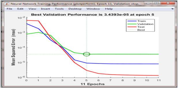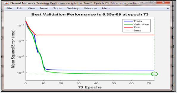Using these parameters, an optimum neural network architecture was generated. The network training diagram generated for the prediction of Brinell hardness number (BHN), heat input (HI) and cooling rate (CR) using back propagation neural network is presented in (Figures 1-3) respectively.

From the performance plot of (Figure 1), no evidence of over fitting was observed. In addition, similar trend was observed in the behaviour of the training, validation and testing curve which is expected since the raw data were normalized before use. Lower mean square error is a fundamental criterion used to determine the training accuracy of a network. An error value of 3.4393e-05 at epoch 5 is an evidence of a network with strong capacity to predict Brinell hardness number. From the performance plot of (Figure 2), no evidence of over fitting was observed. In addition, similar trend was also observed in the behaviour of the training, validation and testing curve which is expected since the raw data were normalized before use. Lower mean square error is a fundamental criteria used to determine the training accuracy of a network. An error value of 6.3500e-09 at epoch 73 is an evidence of a network with strong capacity to predict heat input. From the performance plot of (Figure 3), no evidence of over fitting was observed. In addition, similar trend was observed in the behaviour of the training, validation and testing curve which is expected since the raw data were normalized before use. Lower mean square error is a fundamental criterion used to determine the training accuracy of a network. An error value of 0.00034858 at epoch 40 is an evidence of a network with strong capacity to predict cooling rate.

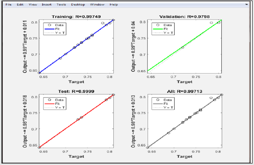
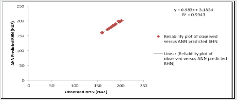
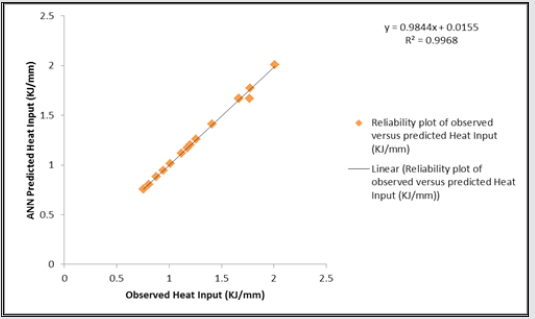
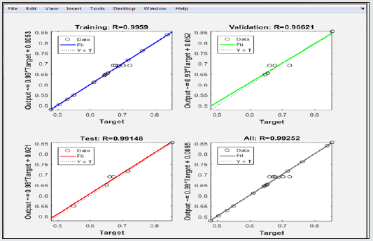
The regression plot which shows the correlation between the input variables (current, voltage and welding speed) and the target variable Brinell hardness number (BHN), heat input (HI) and cooling rate (CR) coupled with the progress of training, validation and testing is presented in (Figures 4,5,6) respectively. Based on the computed values of the correlation coefficient (R) as observed in (Figures 4,5,6), it was concluded that the network has been adequately trained and can be employed to predict the Brinell hardness number, heat input and cooling rate. To test the reliability of the trained network, the network was thereafter employed to predict its own value of Brinell hardness number, heat input and cooling rate using the same set of input parameters (current, voltage and welding speed) generated from the central composite design. Based on the observed and the predicted values, a regression plot of outputs was thereafter generated and presented in (Figures 7,8,9) respectively. Based on the results of Figures (Figures 7,8,9), the following inference were drawn.

a. Coefficient of determination (r2) values of 0.9943 as observed in (Figure 7) was employed to draw a conclusion that the the trained network can be used to predict the Brinell hardness number (BHN) beyond the scope of experimentation.
b. Coefficient of determination (r2) values of 0.9968 as observed in (Figure 8) was employed to draw a conclusion that the the trained network can be used to predict the Heat input (HI) beyond the scope of experimentation.
c. Coefficient of determination (r2) values of 0.9851 as observed in (Figure 9)was employed to draw a conclusion that the the trained network can be used to predict the cooling rate (CR) beyond the scope of experimentation.

Conclusion

Artificial Neural Network (ANN) is gradually gaining general acceptability as one of the most versatile predictive tools of the 21st century. Its application and usefulness especially in the process industry cannot be over emphasized. In this study, the network has successfully been utilized to predict weld variables effectively. The high coefficient of determination obtained from the regression plot of observed and predicted variables can account for the successful implementation of Artificial Neural Network.

References

1. Navid N, Jill U (2016) Finite Element Analysis for Thermal Analysis of Laser Cladding of Mild Steel with P420 Steel Powder; Proceedings of the ASME 2016 International Mechanical Engineering Congress and Exposition. ASME 123-136.
2. Vikram S (2013) An Investigation for Gas Metal Arc Welding Optimum Parameters of Mild Steel AISI 1016 using Taguchi‟s Method. IJEAT 2(6): 407-409.
3. Setiono R, Wee KL, Zurada JM (2002) Extraction of rules from artificial neural networks for nonlinear regression, Published in.IEEE Transactions on Neural Networks 13(3): 564 -577.
4. Sreeraj P, Kannan T, Subhasis M (2013) Optimization of weld bead geometry for stainless steel cladding deposited by GMAW. AJER 2(5): 178-187.
5. Sinan MT, Beytullah E, Asude A (2011) Prediction of adsorption efficiency for the removal of Ni (II) ions by zeolite using artificial neural network (ANN) approach, Fresenius Environmental Bulletin 20(12): 3158-3165.
6. Kimchi M, Sun X, Stephens EV, Khaleel MA, Shao H (2002) Resistance Spot Welding of Aluminum Alloy to Steel with Transition Material from Process to Performance Part I: Experimental Study. Welding Journal pp. 188-195.
7. Tarun KJ, Bhuvnesh B, Kulbhushan B, Varun S (2014) Prediction and Optimization of Weld Bead Geometry in Gas Metal Arc Welding Process using RSM. International Journal of Science, Engineering and Technology 2(7): 34-42.