Visualization of Voxel Volume Emission and Absorption of Light in Medical Biology Volume 1 - Issue 3

Afeez Mayowa Babalola¹*, Lateef Adebayo Babalola¹, Maxwell Obubu² and Taofikat Abidemi Azeez³

• ¹ Department of Statistics, University of Ilorin, Ilorin, Nigeria
• ²Department of Statistics, Nnamdi Azikiwe University, Awka, Nigeria
• ³ Department of Mathematics, University of Ilorin, Ilorin, Nigeria

Received: March 18, 2019;   Published: March 27, 2019

*Corresponding author:Afeez Mayowa Babalola, Department of statistics, university of Ilorin, Ilorin, Nigeria

DOI: 10.32474/CTBB.2019.01.000114

Abstract PDF

---

Abstract

Background: The study is mainly focused on visualization technique that gives a 3D impression of the whole data set without segmentation. The underlying model is based on the emission and absorption of light that pertains to every voxel of the view volume. The algorithm simulates the casting of light rays through the volume from preset sources. It determines how much light reaches each voxel on the ray and is emitted or absorbed by the voxel. Then it computes what can be seen from the current viewing point as implied by the current placement of the volume relative to the viewing plane, simulating the casting of sight rays through the volume from the viewing point.

Keywords: Visualization; Volume Rendering; Volren; Voltex Spinal; Amira; Medical Imaging

Introduction

Volume rendering using computer graphics in scientific visualization is a set of techniques used to display a 2D projection of a discreetly sampled 3D data set, typically a 3D data field, a typical 3D data set is a set of 2D slice images acquired by a CT, MRI or micro CT scanner. Usually these are acquired in a regular pattern (e.g. one slice per millimeter) and usually in a regular pattern have a regular number of image pixels. This is an example of a regular volumetric grid with each volume element or voxel represented by a single value that is obtained by sampling the voxel’s immediate area. Volume rendering involves the following steps: forming an RGBA volume from the data, reconstructing a continuous function from this discrete set of data and projecting it from the desired point of view onto the 2D viewing plane (the output image). Volume rendering is distinguished from thin slice tomography presentations and is also generally distinguished from projections or projections. Fishman et al. [1] Technically, however, when viewed on a 2-dimensional display, all volume renderings become projections, making the difference between projections and volume renderings a little vague. Nevertheless, there is a mix of coloring [2] and shading in the epitomes of volume rendering models to create realistic and/or observable representations.

In order to render a 2D projection; a camera must first be defined in space relative to the volume of the 3D data set. You also need to define each voxel’s opacity and color. Usually this is defined using a transfer function RGBA (for red, green, blue, alpha) that defines the RGBA value for any voxel value. For example, by extracting iso surfaces (surfaces of equal values) from the volume and rendering them as polygonal meshes or rendering the volume directly as a data block, a volume can be viewed. A common technique for extracting an iso surface from volume data is the marching cubes algorithm. Rendering direct volume is a computationally intensive task that can be accomplished in several ways. A direct volume renderer [3,4] requires an opacity and a color mapping of each sample value. This is done with a “transfer function” that can be a simple ramp, a linear function in pieces, or an arbitrary table. Once converted to an RGBA (red, green, blue, alpha) value, the result of the compound RGBA is projected on the appropriate frame buffer pixel. The way this is done is dependent on the technique of rendering. It’s possible to combine these techniques. For example, to draw the aligned slices in the off-screen buffer, a shear warp implementation could use texturing hardware. The technique of volume ray casting can be derived directly from the rendering equation. The volume ray casting technique can be derived directly from the equation of rendering. It delivers very high-quality results, usually considered to deliver the best quality of the image. Volume ray casting is classified as an image-based volume rendering technique, as the computation emanates from the output image, not the input volume data as is the case with object-based techniques. A ray is generated for each desired pixel of the image in this technique. Using a simple camera stacked to form a 3D model using multiple X-ray tomographs (with quantitative calibration of mineral density). Volume rendered a forearm CT scan with different muscle, fat, bone, and blood color schemes.

Basics for Medical Volume Rendering

Computer graphics traditionally represented a model as a set of vectors displayed on graphic vector displays. By introducing raster displays, polygons became the basic primitive rendering, where a model’s polygons were rasterized into pixels representing the frame buffer’s compounds. Compared to surface data that only determines an object’s external shell, volume data is used to describe a solid object’s internal structures. A volume is a standard 3D array of voxels, data values. The three-dimensional array can also be viewed as a stack of two-dimensional data value arrays and as an image (or slice) each of these two-dimensional arrays, where each of the data values represents a pixel (Figure 1). The slice-oriented, traditional way doctors look at a volumetric dataset motivates this alternative view. It is referred to as a matrix V = xxyy z with X rows, Y columns and Z slices, representing a discrete grid of volume elements (or voxels) v {1, . . ., X} {1, . . ., Y}} {1, . . ., Z}. For each voxel we refer to I(v): N 3 as its gray value, reflecting, for example, the x-ray intensity in CT volume data. Of course, in certain specific fields (e.g. computational fluid dynamics), the voxel value can be a vector to represent the object properties. Every voxel is characterized by its 3D grid position. MRI (Magnetic Resonance Imaging) and CT-scanner (Computed-Tomography) medical volume data are typically anisotropic with an equal sampling density in x and y direction but a higher density in z direction. These data sets V are the basis for our assessment of volume rendering algorithms.

Optical Model for Volume Rendering

The basic objective of volume rendering is to find a good approximation of the low albedo volume rendering optical model that expresses the relationship between volume intensity and opacity function and image plane intensity. We describe a typical physical model in this section that is based on volume rendering algorithms. Our intention is to explain theoretical bases on which algorithms are based for volume rendering. Physical optical models are provided by the theory of radiative transport, which attempts to view a volume as a particle-populated cloud. By considering the different phenomena at work, light transport is studied. Particles can either disperse or absorb light from a source (6). When particles emit light themselves, there may be a net increase. Models that take all the phenomena into account tend to be very complicated. Much simpler local models are being used in practice. Therefore, most standard volume rendering algorithms approximate an integral volume rendering equation (VRI) [5,6] by:

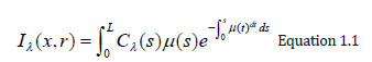
Where the amount of light of wavelength π from ray direction r received at x on the image plane is Iπ, the length of the ray r is L, the density of volume particles receiving light from all surrounding light sources is μ and reflecting this light to the observer according to their specular and diffuse material properties, the light of wavelength π is reflected and/or reflected and/or reflected.

The equation 1.1 cannot generally be calculated analytically. Most volume rendering algorithms therefore obtain an Equation 1.1 numeric solution in practical uses by using a zero-order quadrature of the inner integral together with an exponential firstorder approximation. The outer integral is also solved by a finite sum of uniform samples. Then we obtain the familiar composite equation [7]:

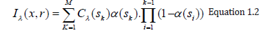
Local color values derived from the illumination model are α(s_k) opacity samples along the ray and Cπ(s_k). This term is referred to as discrete VRI (DVRI), where α= 1.0 − transparency opacity. Equation 1.2 is a common theoretical framework for all algorithms for volume rendering. In discrete intervals, all algorithms obtain colors and opacity along a linear path and compose them in front to back order. The algorithms, however, can be distinguished by the process in which the colors Cπ (s_k) and opacities α (s_k) are calculated at each interval k and how wide the interval widths are selected [6]. C and α are now functions for transfer, commonly used as search tables. The raw volume densities are used to index the color and opacity transfer functions, making it possible to express the fine volume data details in the final image using various transfer functions.

Amira Computer Program

Amira is a system for visualizing, analyzing and modeling 3D data. It allows you to view scientific data sets from different fields of application, e.g. medicine, biology, biochemistry, microscopy, biomedicine, bioengineering. It is possible to explore, analyze, compare and quantify 3D data quickly. 3D objects can be represented as image volumes or geometric surfaces and grids suitable for numerical simulations, particularly as triangular surfaces and tetrahedral volumetric grids. Amira provides methods for generating such grids from voxel data representing a volume of images and includes an interactive 3D viewer for general purposes. Amira is a powerful, multi-faceted software platform that visualizes, manipulates and understands life science and bio-medical data from all sources and modalities. Initially known and widely used as the preferred 3D visualization tool in microscopy and biomedical research, Amira has become an increasingly sophisticated product, providing powerful capabilities for visualization and analysis in all fields of visualization and simulation in Life Science.

Aims and Objectives

The aim of this Research is

To determine the meaning of the study, the opacity and color of each voxel must be defined, and the 3D images visualized.

Objectives of the Study are

A. Develop an image visualization volume rendering technique to overcome the problems of accurate surface representation in iso surface techniques.

B. Visualize and display the true image color.

Data Source

Data collected For the purpose of this research is a total of four (4) patients voxel data was collected from Kwara Diagnostic Center Ilorin, Kwara Nigeria. The AMIRA IMAGING software (Version 5.33) was used for the visualization technique that gives a 3D impression of the whole data set without segmentation. A specific modular software architecture, where multiple related modules are organized into different packages, ensures the flexibility and extensibility of amira. Each package exists in the form of a shared library (or Windows DLL) that is linked at runtime to the main program.

Methodology

The last 15 + years of computer graphics and applications have proven the value of volume rendering techniques in general and interactive rendering applications across domains for scientific visualization: from medical imaging to geophysics to transport security. There is a healthy community of researchers working on volume rendering models and algorithms; their efforts are focused largely on different approaches to lighting, rendering techniques, and handling large datasets [8]. However, one issue that is rarely addressed is volume rendering reproducibility. There are many reasons why reproducibility is hard- from hardware and software architectures to network protocols to data types and sizes growth, re-implementing and recreating even common volume rendering algorithms on a shifting, babelized and proprietary technological landscape is difficult. However, its mission-critical’ in the knowledge enterprise that data becomes verifiable information and that this information is interoperable across platforms between systems and portable.

We broadly use the term ‘ enterprise’ to describe any organization (research, clinical, industrial) that requires scalable and efficient access to data by diversified workers. First let’s consider as a scientific research undertaking the following examples from academia: a perceptual study on the value of a new volume rendering algorithm for stereo depth discrimination, and a 3DUI study on volumetric data surgical planning. In both of these cases, the study’s scientific findings are valid only in so far as they can be repeated: that is, they can be implemented, run and evaluated independently. Several cases of use are evident in the IEEE VR 2010 Medical Virtual Workshop for example, The stimulus generating parameters (views) include transformations of camera and object, lighting equations, ray-casting algorithms, properties of mesh and isosurfaces materials, clipping planes, etc. All must share a conceptual interoperability and equivalence irrespective of the proprietary application, rendering library or display hardware used.

Volumetric medical image rendering is a method of extracting meaningful information from a three-dimensional (3D) dataset, making it possible for radiologists as well as physicians and surgeons to better understand the processes of disease and anatomy. Since the advent of computerized imaging modalities such as computed tomography (CT), magnetic resonance imaging (MRI), and positron emission tomography (PET) in the 1970s and 1980s, medical images have evolved from two-dimensional projections or slice images to fully isotropic three-and even four-dimensional images such as those used in dynamic cardiac studies. This evolution has made the traditional means of viewing such images (the view-box format) inappropriate to navigate the large data sets that comprise the typical 3D image today. While an early CT slice (320320 pixels) contained about 100k pixels, the current 5123 CT image contains about 1,000 times the amount of data (or about 128 M pixels) [9].

This huge increase in image size requires a more effective way of manipulating and visualizing these datasets. [10,11] This is necessary on two fronts: the radiologist must navigate the data to make a diagnosis, while the surgeon needs a precise 3D patient representation (and related pathology) to plan a therapeutic procedure [12]. In order to appreciate the full three-dimensional attributes of the data, the individual voxels in the dataset must be mapped to the viewing screen to maintain their 3D relationships while making their screen appearance meaningful to the observer [13] (Peters TM 2006). The shift from traditional axial sections to primary 3D volume visualization can provide better visualization of anatomical structures and thus enhance the performance of radiologists in efficiently and comprehensively reviewing large medical data sets. Therefore, the confidence of the radiologists in the diagnosis of diseases is increased and patient care is improved.

Direct Volume Rendering (DVR)

Direct Volume Rendering (DVR) idea is to directly obtain a 3D representation of volume data. A semi-transparent light-emitting medium is considered to represent the data. Therefore, it is also possible to simulate gaseous phenomena. DVR approaches are based on physics laws (emission, absorption, dispersal). The volume data is used as a whole (we can see all interior structures and look inside the volume). A direct volume renderer [3,4] requires an opacity and a color mapping of each sample value. This is done with a “transfer function” that can be a simple ramp, a linear function in pieces, or an arbitrary table. Once converted to an RGBA (red, green, blue, alpha) value, the result of the compound RGBA is projected on the appropriate frame buffer pixel. The way this is done is dependent on the technique of rendering. These techniques can be combined. For instance, a shear warp implementation could use texturing hardware to draw the aligned slices in the off-screen buffer. It is possible to use either reverse or forward methods in DVR. Backward methods use algorithms for image space / image order. Pixel by pixel they are performed. Ray casting is an example that will be discussed in detail below [14-19]. use object space/ object order algorithms. These algorithms are performed voxel by voxel and the cells are projected onto the image. Examples for this technique are Slicing, shear-warp and splatting (Figures 2.0 & 2.1).

Volume Ray Casting Model

Ray Casting resembles ray tracing in computer graphics based on the surface. We only deal with primary rays in volume rendering, i.e. no secondary rays are considered for shadows, reflection or refraction. Ray Casting is a technique of natural image order. Since we don’t have any surfaces in DVR, we need to step through the volume carefully. A ray is cast into the volume and at certain intervals the volume is sampled. Usually the sampling intervals are equidistant, but they do not need to be (e.g. sampling of importance).

The ray starts at the center of the camera’s projection (usually the eye-point) and passes through the image pixel on the imaginary image plane floating between the camera and the rendering volume. To save time, the ray is clipped by volume boundaries. Then the ray is sampled throughout the volume at r;2regular or adaptive intervals. At each sample point, the data is interpolated, the transfer function is applied to form a RGBA sample, the sample is composed on the ray’s accumulated RGBA, and the process is repeated until the ray exits the volume. The RGB color is converted to an RGB color and deposited in the appropriate pixel of the image. For each pixel on the screen, the process is repeated to form the completed image. At each sampling location, a sample is interpolated/reconstructed from the voxel grid. Popular filter is nearest neighbor (box), trilinear, or more sophisticated (Gaussian, cubic spline) [20].

Volumetric Ray Integration: The rays are casted through the volume. Color and opacity are accumulated along each ray (compositing) (Figure 2.2 & 2.3).

A. How is color and opacity determined at each integration step?

B. Opacity and (emissive) color in each cell according to classification

C. Additional color due to external lighting: according to volumetric shading (e.g. Blinn Phong) How can the compositing of semi-transparent voxels be done? Physical model: emissive gas with absorption

D. Approximation: density-emitter-model (no scattering)

E. Over-operator was introduced by Porter [Porter-1984- CDI]: C ^out=(1−α) C ⁱⁿ +αC,

C(i)ⁱⁿ = C (i−1)^out

(Figure 2.4) A front-to-back-strategy is also possible: C ^out = C ⁱⁿ + (1−α ⁱⁿ) αC, α^out=αⁱⁿ + (1−α ⁱⁿ) α This approach causes the need to maintain α (Figure 2.5).

There are several traversal strategies:

A. Front-to-back (most often used in ray casting)

B. Back-to-front (e.g. in texture-based volume rendering)

C. Discrete (Bresenham) or continuous (DDA) traversal of cells

Texture Based Volume Rendering

Texture-based volume rendering is an approach to generate an image viewed with different camera parameters using scene information extracted from a set of reference images. The rendering speed of this approach depends only on image size instead of scene complexity, and complex hand-made geometric models are not required. Further these techniques take advantage of functionality implemented on graphics hardware like Rasterization, Texturing and Blending [21-24] (Figures 2.6 & 2.7).

Volume Segmentation

Image segmentation is a manual or automatic procedure that can be used to select large portions of the volume that one considers uninteresting before rendering can significantly reduce the amount of calculations to be made by casting rays or blending texture [25]. For n sequentially indexed voxels, this reduction can be as much from O(n) to O (log n). Volume segmentation also has significant performance advantages for other algorithms for ray tracing. Subsequently, volume segmentation can be used to highlight interesting structures.

Bounding Box

Setting the Bounding Box

To visualize its bounding box, the Bounding Box module can be connected to any spatial data object. A data object’s bounding box includes its scope in 3D. More accurately, the minimum and maximum coordinates in the x, y, and z directions are determined. Amira usually does not know the physical dimensions of the images when loading a series of bitmap images. Hence an Image Read Parameters dialog appears which prompts you to enter the bounding box’s physical extent. Alternatively, you can set the size of a single voxel. In Amira, an object’s bounding box is the smallest rectangular, axis-aligned volume in the object’s 3D space [26-28]. Note that a uniform data set bounding box extends from the center of the first voxel to the center of the last one in Amira.

Otho Slice

Choose the Entry called Orthoslice from the Popup Menu of the Di com Data Set

Now a 2D slice is displayed in the viewer window through the optical lobe. A slice oriented perpendicular to the z-direction is initially displayed and centered within the volume of the image. The number of slices is 0, 1, 2, and so on. Both the slice number and the orientation are Ortho Slice module parameters. You must select the module to change these parameters. With regard to the green data icon, this is done by clicking with the left mouse button on the Ortho Slice icon. By the way, the Ortho Slice icon is orange in contrast to the Bounding Box, indicating that this module can be used to clip.

select the Ortho Slice Module

Now you should see in the Properties Area different buttons and sliders, ordered in rows. Each row is a port that allows you to adjust a specific parameter of the control. Usually at the beginning of a row the name of a port is printed. The port called Slice Number, for example, allows you to change the number of the slice via a slider.

Select Different Slices using the Slice Number Port

Ortho Slice displays axially oriented slices, i.e. perpendicular to the z-direction, by default. The module, however, can also extract slices perpendicular to x-and y-direction from the image volume. Sagittal and coronal (these are standard phrases used in radiology) are sometimes referred to as these two alternatives.

Volren

Volume Rendering is a visualization technique that gives a 3D impression of the whole data set without segmentation. The underlying model is based on the emissL2ion and absorption of light that pertains to every voxel of the view volume. The algorithm simulates the casting of light rays through the volume from preset sources. It determines how much light reaches each voxel on the ray and is emitted or absorbed by the voxel. Then it computes what can be seen from the current viewing point as implied by the current placement of the volume relative to the Visualizing 3D Images viewing plane, simulating the casting of sight rays through the volume from the viewing point [29].

A. You can choose between two different methods for these computations: maximum intensity projections or an ordinary emission absorption model.

B. Remove all objects in the Pool other than the di com data record.

C. Connect a Voltex module to the data.

D. Select the data icon and read off the range of data values printed on the first info line (22...254).

E. Select the Voltex module and enter the range in the Color map port.

F. Press the Apply button in order to perform some texture preprocessing which is necessary for visualizing the data.

By default, emission absorption volume redering is shown. The amount of light being emitted and absorbed by a voxel is taken from the color and alpha values of the color map connected to the Voltex module. In our example the color map is less opaque for smaller values. You may try to set thK6e lower bound of the color map to 40 or 60 in order to get a better feeling for the influence of the transfer function. In order to compute maximum intensity projections, choose the mip option of port Options. Internally, the voltex module makes heavy use of OpenGL texture mapping. Both texture modes, 2D and 3D, are implemented. 3D textures yield slightly better results. However, this mode is not supported by all graphics boards. The 3D texture mode requires you to adjust the number of slices cut through the image volume. The higher this number the better the results are [30]. Alternatively, 2D textures can be used for volume rendering. In this case, slices perpendicular to the major axes are used. You may observe how the slice orientation changes if you slowly rotate the data set. The 2D texture mode is well suited for midrange graphics workstations with hardware accelerated texture mapping. If your computer does not support hardware texture mapping at all, you should use visualization techniques other than volume rendering.

a. Make sure the mip button of port Options is unchecked.

b. If 3D texture mode is enabled, choose about 200 slices.

c. Click with the right mouse button on port Color map and choose volren Red. icol.

d. Set Lookup to RGBA and change the min and max values of the color map to 40 and 150.

e. Finally, press Apply in order to initialize the Voltex textures. Whenever you choose a different color map or change the min and max values of the color map, you must press the Apply button again. This causes the internal texture maps to be recomputed. An exception are SGI systems with Infinite Reality graphics. On these platforms a hardware-specific OpenGL extension is exploited, causing color map changes to take effect immediately.

Animating an Orthoslice Module

Note that there is a port called Slice Number in the Ortho Slice module. If you change that slider’s value, in the viewer you see the plane moving. Now let’s use the Demo Maker module and the Demo Director GUI as our first exercise to animate this slider. Use the right click in the pool to add a Demo Maker module to the pool and select Create Animation / Demo Maker [31].

Result and Discussion

Kwara Diagnostic Center Ilorin, Kwara Nigeria. We collected a total of four (4) voxel patient data. Each voxel has its own structure as shown in the figures below. Data underwent various processes for accurate image display and visualization. Moreso, it shows how the orthogonal slices differ from the volren images.

Modelling Of Human Patient Skull

(Figure 3.1) A student could begin to explore the skull model with a skin surface image of the head. As the first step, one could simply cut into the head and explore the appearing section. However, an anatomist would prefer to remove the tissue layer by layer. This easily can be simulated by “selective cutting”. Since the cut surfaces exhibit the original intensity values, the scene has the appearance of an actual dissection. The crucial advantage of the computer model is to improve the contrast of the image. As seen in Figures 3.1. The corresponding region can be colored as well. Thus, questions about the nature of the visible objects can be answered easily [32]. The advantage of the Volren image over the ortho slice image as seen in Figure 3.1 is that, it determines how much light reaches each voxels on the ray and is emitted or absorbed by the voxel. The white portion of the orthogonal slice image indicates that, there was no blood circulation in that portion.

Figure 3.2 shows how the patient spine was been modeled to depicts its true color by using ortho slice and volren. With amira MR images of the spine are clearer and more detailed than images obtained with other imaging methods. In Figure 3.2 above, it shows the abnormalities, injuries and diseases in the spinal region that may not be seen with other imaging methods. With Amira, MRI is the best available modality to visualize spinal cord and nerves. After undergoing different process e.g, bounding box, ortho slice, volren am and animation MRI enables the discovery of abnormalities that might be obscured by bone with other imaging methods.

The differences of Amira and other imaging software’s are;

A. With Amira, MRI is very useful for evaluating spinal injuries. It is especially helpful for diagnosing or ruling out acute compression of the spinal cord when the clinical examination shows muscle weakness or paralysis. MRI is the best modality available for evaluation of ligament injuries.

B. Is able to detect subtle changes in the vertebral column that may be an early stage of infection or tumor. The procedure is more sensitive than CT scanning for evaluating tumors, abscesses and other soft tissue masses near the spinal cord. Is the preferred technique in evaluating for potential complications of surgery, including bleeding, scarring, infection and re-appearance of a herniated disk?

Modeling of a Patient Human Sagital

From Figure 3.3 above, you will notice that the sagittal midline of the brain is one of the most important sectional planes in neuroimaging. A good working knowledge of the normal neuro anatomy of the sagittal midline is essential so that the subtle abnormalities that may manifest here can be recognized. We discovered that neuroembryological development of the brain results in a striking symmetry that is evident throughout the majority of the brain. The sagittal midline in neuroimaging provides a unique opportunity to observe in a single slice, the continuity of the cerebra spinal fluid pathways, to observe if there are any abnormalities of the brain stem and diencephalon such as agenesis or hypoplasia and to observe if there is any displacement of the midline [33] (Figure 3.4).

Conclusion

After Amira, a 3D visualization and geometry reconstruction system, we presented the general design concepts. We also provided an overview of the various techniques and algorithms used in this system. It has been shown that the combination of different concepts such as object orientation, a simple and well-structured user interface, highly interactive component integration such as the segmentation editor, intuitive 3D interaction techniques, A powerful scripting interface and a wide range of advanced and innovative visualization and data processing algorithms have resulted in a powerful software system that can be used in many medical, biological and other scientific disciplines. The relationship between the orthogonal slices and volren is one of the significant findings that emerged from this study. We noticed that we could determine the true colors of images in 3D by using Volren in Amira.

Recommendations

For properly addressing the above limitations, my recommendations are as follows:

a. It is recommended that no much hypothesis be made for more and more accurate results, as this will help reduce error.

b. Courses related to modeling and simulations should be incorporated as a matter of urgency as part of our curriculum of tertiary education. As we all know, especially in scientific research, the world is digitizing, you would agree with me that most research work is done using software such as MATLAB, AUTOCAD, and so on.

References

1. Fishman Elliot K, Ney Derek R, Heath David G, Corl Frank M, Horton Karen M, et al. (2006) Volume Rendering versus Maximum Intensity Projection in CT Angiography: What Works Best, When, and Why. Radio Graphics 26 (3): 905-922.
2. Silverstein Jonathan C, Parsad Nigel M, T sirline Victor (2008) Automatic perceptual color map generation for realistic volume visualization. Journal of Biomedical Informatics. 41 (6): 927-935.
3. Marc Levoy (1988) Display of Surfaces from Volume Data. IEEE CG&A 8(3): 29-37.
4. Drebin Robert A, Carpenter Loren, Hanrahan Pat (1988) Volume rendering. ACM SIGGRAPH Computer Graphics. 22 (4): 65-74.
5. Max N, Hanrahan P, Crawfis R (1990) Area and volume coherence for efficient visualization of 3D scalar functions. ACM SIGGRAPH Computer Graphics 24(5): 27-33.
6. Meissner M, J Huang, D Bartz, K Mueller, R Crawfis (2000) A Practical Evaluation of Popular Volume Rendering Algorithms. In IEEE/ACM Symposium on Volume Visualization, Salt Lake City, Utah, USA p. 81-90
7. Levoy M (1990) Efficient Ray Tracing of Volume Data. ACM Transactions Computer Graphics and Applications 9(3): 245-261.
8. Jnsson D, Sundn E, Ynnerman A, Ropinski T (2012) Interactive volume rendering with volumetric illumination. In Eurographics 2012 -State of the Art Reports, p. 53-74.
9. Preim B, Bartz D (2007) Visualization in Medicine: Theory, Algorithms, and Applications (The Morgan Kaufmann Series in Computer Graphics). (1st edn). Morgan Kaufmann, San Mateo, pp. 680.
10. Robb RA, Hanson DP (2006) Biomedical image visualization research using the visible human datasets. Clin Anat 19(3): 240-253.
11. Linsen L, Hagen H, Hamann B (2007) Visualization in Medicine and Life Sciences. (Mathematics and Visualization) (1st edn). Springer, Berlin, Germany.
12. Vidal F, F Bello, KW Brodlie, DA Gould, NW John, et al (2006) Principles and applications of computer graphics in medicine. Comput Graph Forum 25(1): 113-137.
13. Udupa J, Herman G (1999) 3D imaging in medicine. (2nd edn). CRC, pp. 384.
14. Babalola AM, Obubu M, Otekunrin OA, Obiora-Ilono H (2018) Selection and Validation of Comparative Study of Normality Test. American Journal of Mathematics and Statistics 8(6): 190-201.
15. Babalola AM, Obubu M, George OA, & Ikediuwa CU (2018) Reprospective Analysis of Some Factors Responsible for Infant Mortality in Nigeria: Evidence from Nigeria Demographic and Health Survy (NDHS). American Journal of Mathematics and Statistics 8(6): 184-189.
16. Engel Klaus, Kraus Martin, Ertl Thomas (2001) High-quality preintegrated volume rendering using hardware-accelerated pixel shading. Proceedings of the ACM SIGGRAPH/EUROGRAPHICS workshop.
17. Hibbard W, Santek D (1989) Interactivity is the key. Chapel Hill Workshop on Volume Visualization, University of North Carolina, Chapel Hill, USA, p. 39-43.
18. https://en.m.wikipedia.org/wiki/Volume_rendering
19. https://graphics.ethz.ch/teaching/former/scivis_07/Notes/stuff/ StuttgartCourse/VIS-Modules-06-Direct_Volume_Rendering.pdf
20. https://www.cc.gatech.edu/scivis/tutorial/linked/volrend.html
21. Huang Jian (Spring 2002) Splatting. (http://web.eecs.utk.edu/~huangj/ CS594S02/splatting.ppt) (PPT).
22. Jianlong Zhou, Klaus D T onnies (2003) 1 State of The Art for Volume Rendering. Institute for Simulation and Graphics University of Magdeburg, Magdeburg, Germany.
23. Lacroute Philippe, Levoy Marc (1941) Fast Volume Rendering Using a Shear-warp Factorization of the Viewing Transformation” (http:// graphics.stanford.edu/papers/shear/). Proceedings of the 21st Annual Conference on Computer Graphics and Interactive Techniques. SIGGRAPH New York, USA: ACM, pp. 451-458.
24. Lum E, Wilson B, Ma K (2004) High-Quality Lighting and Efficient Pre- Integration for Volume Rendering. In Eurographics/IEEE Symposium on Visualization.
25. Max N (1995) Optical Models for Direct Volume Rendering. IEEE Transactions on Visualization and Computer Graphics 1(2): 99-108.
26. Obubu M, Babalola AM, Ikediuwa CU, Amadi PE (2019) Parametric Survival Modeling of Maternal Obstetric Risk; a Censored Study. American Journal of Mathematics and Statistics 9(1): 17-22.
27. Obubu M, Babalola AM, Ikediuwa CU, Amadi PE (2018) Modelling Count Data; A Generalized Linear Model Framework. American Journal of Mathematics and Statistics 8(6): 179-183.
28. Obubu M, Babalola AM, Ikediuwa CU, Amadi PE (2019) Biometry Investigation of Malaria- Disease, Mortality and Modelling; an Autoregressive Integrated Approach. American Journal of Mathematics and Statistics 9(1): 11-16.
29. Pfister Hanspeter, Hardenbergh Jan, Knittel Jim, Lauer Hugh, Seiler Larry (1999) The Volume Pro real-time ray-casting system. Proceedings of the 26th annual conference on Computer graphics and interactive techniques -SIGGRAPH.
30. Polys N, Johnm N (2010) In IEEE VR 2010 Workshop on Medical Virtual Environments. http://ww’w.hpv.cs.bangor.ac.uk/vr10-med.
31. Sherbondy A, Houston M, Napel S (2003) Fast volume segmentation with simultaneous visualization using programmable graphics hardware. In Proceedings of IEEE Visualization, pp. 171-176.
32. Sielhorst T, Feuerstein M, Navab N (2008) Advanced medical displays: A literature review of augmented reality. J Display Technol 4(4): 451-467.
33. Westover Lee Alan (1991) SPLATTING: A Parallel, Feed-Forward Volume Rendering Algorithm.