The T-R {Generalized Lambda V} Families of Distributions Volume 1 - Issue 2

Clement Boateng Ampadu*

• Carrolton Road, Boston, USA

Received: November 11, 2018;   Published: December 06, 2018

*Corresponding author:Clement Boateng Ampadu, Carrolton Road, Boston, USA

DOI: 10.32474/CTBB.2018.01.000108

Abstract PDF

Abstract

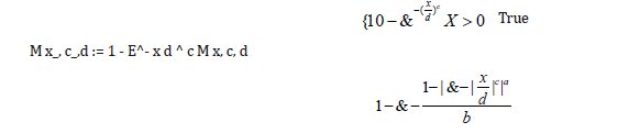
The four-parameter generalized lambda distribution (GLD) was proposed in [1]. We say the GLD is of type V, if the quantile function corresponds to Case(v) in of [2], that is,

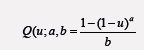
where u 2 (0, 1) and a, b 2 (−1, 0). In this short note, we introduce the T-R {Generalized Lambda V} Families of Distributions and show a sub-model of this class of distributions is significant in modeling real life data, in particular the Wheaton river data, [2]. We conjecture the new class of distributions can be used to fit biological and health data.

Keywords and Phrases: Generalized Lambda Distribution; Exponential Distribution; Weibull Distribution

Contents

a) The T – R {Y} Family of Distributions

b) The New Distribution

c) Practical Significance

d) Open Problem

The T – R {Y} Family of Distributions

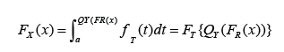
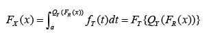
This family of distributions was proposed in [3]. In particular, let T, R, Y be random variables with CDF’s FT (x) = P (T _ x), FR(x) = P (R _ x), and FY (x) = P (Y _ x), respectively. Let the corresponding quantile functions be denoted by QT (p), QR(p), and QY (p), respectively. Also, if the densities exist, let the corresponding PDF’s be denoted by fT (x), fR(x), and fY (x), respectively. Following this notation, the, the CDF of the T – R {Y} is given by

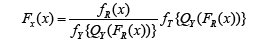
and the PDF of the T-R{Y} family is given by

The New Distribution

Theorem: The CDF of the T-R {Generalized Lambda V} Families of Distributions is given by

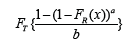
where the random variable R has CDF FR(x), the random variable T with support (0,1) has CDF FT, and a, b 2 (−1, 0) Proof. Consider the integral

and let Y follow the generalized lambda class of distributions of type V, where the quantile is as stated in the abstract

Remark: the PDF can be obtained by differentiating the CDF

Practical Significance

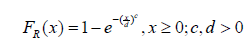
In this section, we show a sub-model of the new distribution defined in the previous section is significant in modeling real life data. We assume T is standard exponential so that FT (t) = 1 − e−t, t > 0 and R follows the two-parameter Weibull distribution, so that

Now from Theorem 2.1, we have the following

Theorem: The CDF of the Standard Exponential-Weibull {Generalized Lambda V}

Families of Distributions is given by

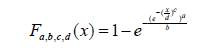
where c, d > 0 and a, b 2 (−1, 0)

By differentiating the CDF, we obtain the following

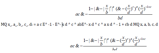
Theorem: the PDF of the Standard Exponential-Weibull {Generalized Lambda V} Families of Distributions is given by

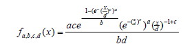
where c, d > 0 and a, b 2 (−1, 0)

Remark: If a random variable B follows the Standard Exponential-Weibull {Generalized

Lambda V} Families of Distributions write

B _ SEWGLV (a, b, c, d)

Open Problem

Conjecture: The new class of distributions can be used in forecasting and modelingn of biological and health data. Related to the above conjecture is the following

Question: Is there a sub-model of the T-R {Generalized Lambda V} Families of Distributions that can fit? [3] (Appendix 1) and (Figures 1-3).

Appendix 1:

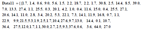
DataQ1 = Flatten Data11; Length DataQ1 72

Min DataQ1 0.1; Max DataQ1 64.

AX1 = Empirical Distribution DataQ1

Data Distribution «Empirical», { 58}

K1 = Discrete Plot [CDF [AX1, x ], {x, 0, 65, (65-0)/58} , Plot Style c {Black, Thick} , Plot Markers c {Automatic, Small} , Filling c None,

Plot Range c All]

(Figure 1)

F1 x_, a_, b: = 1 - 1 - x ^ ab

CDF Weibull Distribution c, d, x

I. Weibull. nb

D 1 - E^ - F1 M x, c, d, a, b, x

PLK1 = Sum Log MQ DataQ1, a, b, c, di, i,1, Length DataQ1;

JK=D [PLK, a];

JK1=D [PLK, b];

JK2=D [PLK, c];

JK3=D [PLK,d];

Find Root JK, JK1, JK2, JK3, a, - 0.11 ,b, - 0.12 , c, 0.9 , d, 11.6

a c – 7.2577, b c – 0.395297, c c 0.776499, d c 657.998

RR = Plot 1 - E^ - F1 M x, 0.776499, 657. 998, - 7.2577, - 0.395297, x, 0, 65, Plot Style c Thick, Blue, Plot Range c All

(Figure 2)

II. Weibull. nb

CMU = Show K1, RR, Plot Range c All

(Figure 3)

Export “CMU.jpg”, CMU CMU.jpg

References

1. Ramberg JS, Schmeiser BW (1974) An approximate method for generating asymmetric random variables. Communications of the ACM 17(2): 78-82.
2. Mahmoud Aldeni, Carl Lee, Felix Famoye (2017) Families of distributions arising from the quantile of generalized lambda distribution. Journal of Statistical Distributions and Applications 4: 25.
3. Ayman Alzaatreh, Carl Lee, Felix Famoye (2014) T-normal family of distributions: a new approach to generalize the normal distribution, Journal of Statistical Distributions and Applications 1:16.