Orthogonal Arrays and Row-Column and Block Designs for CDC Systems Volume 1 - Issue 1

Mahndra Kumar Sharma* and Mekonnen Tadesse

• Department of Statistics, Addis Ababa University, Addis Ababa, Ethiopia

Received: September 06, 2018;   Published: September 20, 2018

*Corresponding author:Mahndra Kumar Sharma, Department of Statistics, Addis Ababa University, Addis Ababa, Ethiopia

DOI: 10.32474/CTBB.2018.01.000103

Abstract PDF

---

Abstract

In this article, block and row-column designs for genetic crosses such as Complete diallel cross system using orthogonal arrays (p², r, p, 2), where p is prime or a power of prime and semi balanced arrays (p^(p-1)/2, p, p, 2), where p is a prime or power of an odd prime, are derived. The block designs and row-column designs for Griffing’s methods A and B are found to be A-optimal and the block designs for Griffing’s methods C and D are found to be universally optimal in the sense of Kiefer. The derived block and rowcolumn designs for method A and C are new and consume minimum experimental units. According to Gupta block designs for Griffing’s methods A,B,C and D are orthogonally blocked designs. AMS classification: 62K05.

Keywords: Orthogonal Array; Semi-balanced Array; Complete diallel Cross; Row-Column Design; Optimality

Introduction

Orthogonal arrays of strength d were introduced and applied in the construction of confounded symmetrical and asymmetrical factorial designs, multifactorial designs (fractional replication) and so on Rao [1-4] Orthogonal arrays of strength 2 were found useful in the construction of other combinatorial arrangements. Bose, Shrikhande and Parker [5] used it in the disproof of Euler’s conjecture. Ray-Chaudhari and Wilson [6-7] used orthogonal arrays of strength 2 to generate resolvable balanced incomplete block designs. Rao [8] gave method of construction of semi-balanced array of strength 2. These arrays have been used in the construction of resolvable balanced incomplete block design. A complete diallel crossing system is one in which a set of p inbred lines, where p is a prime or power of a prime, is chosen and crosses are made among these lines. This procedure gives rise to a maximum of v =p² combination. Griffing [9] gave four experimental methods:

parental line combinations, one set of F₁’s hybrid and reciprocal F₁’s hybrid is included (all v = p² combination)

parents and one set of F₁’s hybrid is included but reciprocal F₁’s hybrid is not (v = 1/2 p^(p+1) combination)

one set of F₁’s hybrid and reciprocal are included but not the parents (v =p^(p-1) combination) and

one set of F₁’s hybrid but neither parents nor reciprocals F₁’s hybrid is included (v = 1/2p^(p-1). The problem of generating optimal mating designs for CDC method D has been investigated by several authors Singh, Gupta, and Parsad [10].

For CDC method A, B and C models of Griffing [9] involves the general combining ability (g ca) and specific combining ability (s_ca) effects of lines. Let n_c denote the total number of crosses involved in CDC method A, B and C and it is desired to compare the average effects or g ca effects of lines. Generally, the experiments of these methods are conducted using either a completely randomized design (CRD) or a randomized complete block (RCB) design involving n_c crosses as treatments. The number of crosses in such mating design increases rapidly with an increase in the number of lines p. Thus, if p is large adoption of CRD or an RCB design is not appropriate unless the experimental units are extremely homogeneous. It is for this reason that the use of incomplete block design as environment design is needed for CDC method A, B and C. Agarwal and Das [11] used n-ary block designs in the evaluation of balanced incomplete block designs for all the four Griffing’s [9] complete diallel cross (CDC) systems. Optimal block designs for CDC method a and b and variance balanced designs for CDC method c have been constructed by Sharma and Fanta [12,13] but their designs consume more experimental units. This call designs for CDC methods A, B and C which consume less experimental units in comparison to their designs and at the same time are A-optimal or optimal. We restrict here to the estimation of general combining ability (g_ca) effects only. For analysis of these designs [12-14].

I in the present paper, we are deriving block and row-column designs for complete diallel cross (CDC) system i.e. methods A, B, C and d through orthogonal arrays and semi balanced arrays. Block designs and row-column designs obtained for methods a consume minimum experimental units and are A-optimal. Block designs obtained for method C are optimal in the sense of Kiefer [15] and consume minimum experimental units but row-column designs are neither A-optimal nor optimal. Conversely block designs and row-column designs obtained for methods B are A-optimal. Block designs obtained for method D are optimal in the sense of Kiefer [15] but row-column designs are neither A-optimal nor optimal. The rest of this article is organized as follows: in section B and C we have discussed universal optimality of designs for 1-way and 2-way settings. In section 4 and 5, we give some definitions of orthogonal array, semi balanced arrays and orthogonally blocked design and relation of orthogonal; array with designs for CDC system and optimality with examples and theorems. In section 6 we give relation of semi-balanced array to CDC system along with theorem and for example.

Model and Estimation in 1-Way Heterogeneity Setting

According to Sharma and Tadesse let d be a block design for a CDC systems experiment involving p inbred lines, b blocks each of size k. This means that there are k crosses in each of the blocks of d. Further, let r_dt and s_di denote the number of replications of cross t and the number of replications of the line i in different crosses, respectively, in d [ t = 1,2, …, n_c; i = 1, 2, …, p]. It is not hard to see that,

n_c = number of crosses and n = bk, the total number of observations. For estimating general combining ability (g_ca) effects of lines, we took the following linear model for the observations obtained from block design d.

where y is an n×1 vector of observations, 1_n is the n×1 vector of ones, △^′₁ is the n × p design matrix for lines and △^′₂ is an n × b design matrix for blocks, that is, the (h,λ)th element of △^′₁ ( respectively, of △^′₁) is 1 if the hth observation pertains to the lth line (respectively, of block) and ois zero otherwise. μ is a general mean, g is a p × 1 vector of line parameters, Β is a b × 1 vector of block parameters and e is an n × 1 vector of residuals. It is assumed that the vector of block parameter, Β is fixed and e is normally distributed with

where I is the identity matrix of conformable order. Using least squares estimation theory with usual restriction , we shall have the following reduced normal equations for the analysis of proposed design d, for estimating the general combining ability (g_ca) effects of lines under model (2.1).

In the above expressions, Gd =△₁ △′₁ = (g_dii´), g_dii = s_di and for i ≠i´, g_dii´ is the number of crosses in d in which the linesi and i´ appear together. N_d= △₁△′₂ = (n_dij), n_dij is the number of times the line i occurs in block j of d and K_d = △₂△′₂ is the diagonal matrix of block sizes. T = △′₁ y and B = △′₂ y are the vectors of lines totals and block totals of order p × 1 and b × 1, respectively for design d. A design d will be called connected if and only if rank (C_d) = p -1, or equivalently, if and only if all elementary comparison among general combining ability (g_ca) effects are estimable using d. We denote by D (p, b, k), the class of all such connected block design {d} with p lines, b blocks each of size k. In section 3, we will discuss Kiefer’s [15] criterion of the universal optimality of D (p, b, k).

Where y is an n × 1 vector of observed responses, μ is the general mean, g, Β and ã are column vectors of p general combining ability (gca) parameters, k row effects and b column effects, respectively, △₁(n× p), △'₂(n× k), △'₃(n×b) are the corresponding design matrices, respectively and e denotes the vector of independent random errors having mean 0 and covariance matrix σ²I_n.LetN_d1 = △₁ △'₂ be the p × k incidence matrix of lines vs rows and N_d2 = △₁ △'₃ be the p × b incidence matrix of treatments vs columns and △₁△'₃= 1_k1_b.Let r_dl denote the number of times the l^th cross appears in the design d, λ = 1, 2, . . . , n_c and similarly s_di denote the number of times the i^th line occurs in design d, i = 1, . . . p. Under (3.1), it can be shown that the reduced normal equations for estimating the g_ca effects of lines with usual restriction , after eliminating the effect of rows and columns, in block design d are

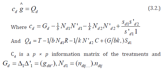
is the number of times line i occurs in row j of d, N_d2= (n_di.t),

n_i.t is the number of times the cross i occurs in column t,

s_d1 is the replication vector of lines in design d,

Q is a p × 1 vector of adjusted treatments (crosses) total,

T is a p × 1 vector of treatment (line) totals,

R is a k × 1 vector of rows totals,

C is a b ×1 vector of columns totals, respectively, in design d,

G is a grand total of all observations in design d,

Now we state the following theorem of Parsad et al. [16] without proof.

Theorem: Let d* ∈ D₁ (p, b, k) be a row - column design and d* ∈ D (p, b, k) be a block design for diallel crosses satisfying

(i) Trace (C_d*) = k-1b {2 k (k-1-2x) + p x (x+1)

(ii) (C_d*) = (p-1)^-1k^--1 b {2 k (k -1-2x) + p x (x+1)} (Ip - p^-1 1p 1′p) is completely symmetric.

Where x = [2k/p], where [z]is the largest positive integer not exceeding z, Ip is an identity matrix of order p and 1p1′p is a p × p matrix of all ones. Then according to Kiefer [15], d*ɛ D₁ (p, b, k) or d*∈ D (p, b, k) is universally optimal and in particular minimizes the average variance of the best linear unbiased estimator of all elementary contrasts among the g_ca effects. Furthermore, using d*ɛ D1 (p, b, k) or d*∈ D (p, b, k) all elementary contrasts among gca effects are estimated with variance.

Some Definitions

Definition 4.1: According to Bose and Bush [17], an r × N matrix A, with entries from a set ∑ of p ≥ 2 elements is called an orthogonal array of strength d, size N, r constraints and p levels if d × N sub matrix of A contains all possible × 1 column vectors with the same frequency λ. The array may be denoted by (N, r, p, d). The number λ may be called the index of the array. Clearly N = λ p^d.

Definition 4.2: According to Rao [8], a (N, r, p) array is said to be a semi-balanced array of strength d if for any selection of d rows α₁, α₂, . . . , α_d, we denote d rows by n(i₁, i₂, . . ., i_d).

(i) n (i₁, i₂, . . ., i_d) = 0 if any two i_j are equal.

Where s represents summation over all permutation of distinct elements i1 , i2, . . ., id.

Definition 4.3: According to Gupta et al. [18], a diallel cross design to be orthogonally blocked if each line occurs in every block r/b time, where r is the constant replication number of the lines and b is the number of blocks in the design.

Relation between Orthogonal Array (p², p⁺¹, p, 2) and Designs for CDC System

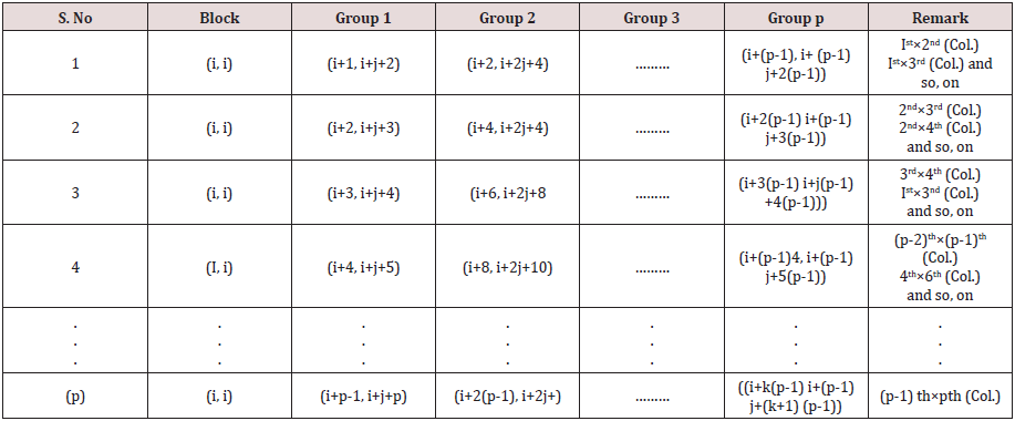
Consider an orthogonal array (p², p+1, p, 2), where p is a prime or power of a prime. If we divide this array into p groups where each group contains p × (p+1) elements and identify the elements of each group as p lines of a diallel cross experiments. Now we perform crosses in any two columns of (p+1) constraints in first group and perform crosses among the lines appearing in the corresponding columns in (p-1) groups, we get p initial columns blocks as given below, which can be developed cyclically mod(p) to get design d1 for diallel cross experiment Griffing’ s method A with p² distinct crosses of p parental lines consisting of p self, 1/2 p (p-1) number of F₁ crosses, and the same number of reciprocal F₁’s with parameter v = p², b = p, k =p , r =1. By this procedure we obtain p^(p+1)/2 designs for diallel cross experiment Griffing’s method A (Table1). Note: All column blocks will be developed cyclically mod (p).

Now considering in d₁ , the cross of the type (i, j) = (j, i), i, j = 1,2, . . . p, we may obtain design d₂ for Griffing’s method B with parameters v = p^(p+1)/2, b =p, k =p, r₁ =1,for cross of the type (i, i) and r₂ =2, for cross of the type (i, j), where i, j = 1, 2, . . ., p, respectively. Considering rows as row blocks in block designs d₁ and d₂ we may also obtain row-column designs d₃ and d₄ for Griffing’s methods A and B with parameters v = p², b = p, k =p, r =1 and v = p^(p+1)/2, b =p, k =p, r₁ =1,for cross of the type (i,i) and r₂ =2, for cross of the type (i, j), where i, j = 1, 2, . . ., p, respectively. If we ignore the crosses of the type (i, i) in d₁, where i = 1, 2, . . . p, we may obtain the block design d₅ for Griffing’s method C with parameters v = p (p-1), b =p, k =p and r =1. Considering the crosses of the type (i, j) = (j, i) in d₅ we may also derive design d₆ for Griffing’s method D with parameters v = p (p-1)/2, b =p, k =p and r =1, where i < j = 1, 2,. . ., p. Considering rows as row blocks in block designs d5 and d6, we may also derive row-column designs d7 and d8 for Griffing’s methods C and D with parameters v = p (p-1), b =p, k =p , r =1 and v = p^(p-1)/2, b =p, k =p and r =1, respectively, The designs d₇ and d₈ are neither optimal nor A-optimal. It is not hard to see that block and row-column designs obtained for Griffing’s methods A and C consume minimum experimental units and in theses designs every cross is replicated only once and each line occurs in every block r/b time, where r is the constant replication number of line and b is the number of blocks in the design. In block designs for Griffing’s methods B and D each line also occurs in every block r/b time. Hence according to Gupta et al. [18] these designs are orthogonally blocked. In an orthogonal design no loss of efficiency on the comparisons of interest is incurred due to blocking. A block design for which N = θ 1p 1′b is orthogonal for estimating the contrasts among gca parameters, where N denotes the line versus block incidence matrix and θ is some constant. For designs d_k ∈ D (p, b, k), where k = 1, 2, 5, and 6 and designs d_k ∈ D₁ (p, b, k), where k = 3, 4, we have n_dkij = 2, for k =1, 2,. . ., 8; i =1, 2, . . .p, j = 1, 2,. . ., p and their information matrices C_dk are as given below.

Where I_p is an identity matrix of order p and 1_p is a unit column vector of ones. Clearly C_dk given by (5.1) is completely symmetric and Trace ( C_dk ) = 2 (p-1)² which is not equal to the upper bound given in (5.3).

Hence the designs d₁, d₂, d₃, and d₄ are not optimal. The information matrix C_dk given by (5.2) is completely symmetric and Trace ( C_dk ) = 2 (p^-1) (p^-2) which is equal to the trace given in (5.3). Hence the designs d₅ and d₆ are optimal in the sense of Kiefer [15] and in particular minimizes the average variance of the best linear unbiased estimator of all elementary contrasts among the gca effects. To prove that the designs d¹, d², d³, and d⁴ are A- optimal, we consider the following criteria. A design d* ∈ D (p, b, k) is said to be A-optimal in D (p, b, k) if and only if Trace ((V_d*)≤Trace(V_d))

Here d* denotes designs d₁, d₂, d₃, and d₄ and d denotes designs d₅ and d₆. The Trace (V_d*) is equal to 1/2 and Trace (V_d*) is which is greater than 1/2.Hence designs d₁, d₂, d₃, and d₄ are an A-optimal.

Remark: The variances of the best linear unbiased estimators of elementary contrasts among gca effects are equal in A-optimal designs and also in optimal designs. It means that all the designs are variance balanced, this fact is particularly attractive to the experimenter, as it enables one to carry out the analysis of the experiment in an extremely simple manner.

Now we state the following theorems.

Theorem: The existence of an Orthogonal Array (p², p⁺¹, p, 2) implies the

existence of different layouts A- optimal incomplete block designs with parameters v = p², b = p, k =p, r =1.

(ii) existence different layouts A- optimal incomplete designs for Griffing’s method B with parameters v = p ^(p+1)/2, b =p, k =p, r₁ =1, for cross of the type (i, i) and r₂ =2, for cross of the type (i, j), where i, j = 1, 2, . . ., p, respectively.

(iii) existence of p^(p-1)/2 row-column designs for Griffing’s [9] methods A and B with parameter v = p², b = p, k =p , r =1 and v = p ^(p+1)/2, b =p, k =p , r₁ =1,for cross of the type (i, i) and r₂ =2, for cross of the type (i, j), where i, j = 1, 2, . . ., p, respectively.

Theorem:- The existence of an Orthogonal Array (p², p⁺¹, p, 2) implies the existence of different layouts optimal incomplete block designs for Griffings [9] methods C and D with parameters v = p^(p-1), b =p, k =p , r =1 and v = p^(p-1)/2, b =p, k =p and r =1, respectively.

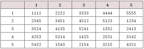
Example: Following Rao [19] we construct an orthogonal array (25,6,5,2) of r_p =5, the 4 orthogonal Latin squares with bordered elements are (Table 2). This arrangement may be expressed in five groups as given below Table 3. The above arrangement is an orthogonal array (25, 6, 5, 2). From the above array we can derive the designs for the four experimental methods described by Griffing [9]. The procedure is explained below.

For Griffing methods A and B, we can take any two columns from first group and corresponding columns from other groups i.e. 2, 3, 4, and 5 and arrange them in columns and then we obtain design for methods A and B. Thus, we may obtain 14 different layouts designs for each method A and method B. We may also obtain 10 different layouts row-column designs for each of these methods A and B.

Remark: - Block and row column designs for methods A and B containing crosses with last column of group 1 are neither A-optimal nor optimal.

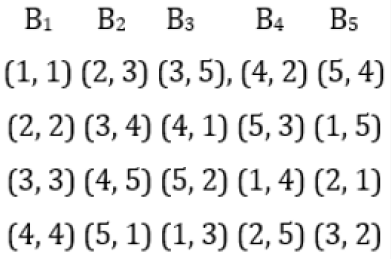
Example: Suppose we take the first two columns from first group and corresponding columns from other groups i.e. 2, 3, 4, and 5. Elements in brackets are considered cross between lines and then we obtain the following design for Griffing’s experimental methods A and B with parameters v = 25, b = 5, k =5, and r =1 and v = 15, b = 5, k =5, and r =1, respectively, with the condition that the cross (i, j) = (j, i) for method (2), where i < j = 1, 2, . . ., 5.

Figure 1 In the above design, considering rows as row blocks, we may we may obtain row-column designs for Griffing’s methods A and B respectively. From the above design we may also derive designs for methods C and D by ignoring the first column and considering (i, j) ≠ (j, i), in other columns, where i, j = 1, 2, 3, 4, and 5, with parameters v = 20, b = 5, k =5, and r =1. In Griffing’s method C design considering (i, j) = ( j, i) , where i< j = 1,2, 3, 4, and 5, we obtain a design for CDC method D with parameters v = 10, b = 5, k =5,and r =2, Thus, from the above array we may obtain 10 different layouts of designs for method C and 10 different layouts of designs for method D.

Relation between Semi-Balanced Array (p^(p-1)/2, p, p, 2) and Designs for CDC System

Consider a semi-balanced (p^(p-1)/2, p, p, 2), where p is an odd prime or power of odd prime. There are (p-1)/2 total sets in a semi-balanced (p^(p-1)/2, p, p, 2). If we identify the elements of semibalanced array as lines of a diallel cross experiment and perform crosses in any two sets among the corresponding lines appearing in the same two sets, we get a mating design for diallel cross experiment involving p lines with v =p²crosses, each replicated once. The mating design can be converted into block design for diallel cross experiment Griffing’s methods A with parameter v = p², b = p, k =p and r =1, considering rows as blocks. In the above design considering the cross (i, j) = (j, i) where i < j = 0, 1, 2, . . ., p, we obtain design for Griffing’s method B with parameters v = p^(p+1)/2, b =p, k =p , r₁ =1,for cross of the type (i, i) and r₂ =2, for cross of the type (i, j), where i, j = 1, 2, . . ., p, respectively.. From block designs obtained for methods A and B we may also obtain row-column designs for Griffing’s methods A and B by considering columns as row blocks with parameters v = p², b = p, k =p and r =1 and v = p^(p+1)/2, b =p, k =p , r₁ =1,for cross of the type (i,i) and r₂ =2, for cross of the type (i, j), where i, j = 1, 2, . . ., p, respectively. From the above mating design deleting the first row and considering (i, j) ≠ ( j, i), where i < j = 0, 1, . . ., p we can also derive designs for methods C, with parameters with parameters v = p (p-1), b =p, k =p , r =1. Considering (i, j) = (j, i), where i, j = 0, 1, . . ., p, we obtain design for Griffing’s method D with parameters v = p^(p-1)/2, b =p, k =p and r =2. Thus, using above techniques, we may obtain different layouts designs for Griffing’s methods A, B, C and D. The information matrices of block designs and row-column designs for methods A and B are same as given in (1). So, block designs and row-column designs for methods A and B are A- optimal. Similarly, the information matrices of designs for methods C and D are the same as given in (1), so designs for methods C and D are universally optimal in the sense of Kiefer [15] and in particular minimizes the average variance of the best linear unbiased estimator of all elementary contrasts among the gca effects. These designs are orthogonally blocked. Now we state the following theorems.

Theorem 1: The existence of semi -balanced array (p^(p-1), p, p, 2) implies the existence of different layouts of A- optimal incomplete block designs and row-column designs for Griffing’s [9] methods A and B with parameters v = p², b = p, k =p and r =1 and v = p^(p+1)/2, b =p, k =p and r =1,respectively, where we consider the cross (i, j) = (j, i) for method B, where i < j = 0, 1, 2, . . ., p.

Theorem 2: The existence of Semi -Balanced Array (p (p-1), p, p, 2) implies the existence of different lay outs of optimal incomplete block designs v = p^(p-1), b =p, k =p and r =1 and v = p^(p-1)/2, b=p, k=p and r=2, respectively, for Griffing’s [9] methods C and D.

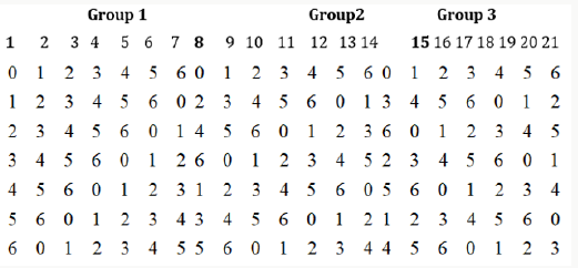
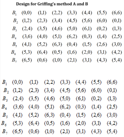
Example. If p =7, the residue classes 0, 1, . . . , 6 (mod7) form a field . We write the 7 elements of GF (7) as 0, ±1, ±2, ±3 and hence the key sets are, using the formula (7.1), where

(0, 1, 2, 3, 4, 5, 6), (0, 2, 4, 6, 1, 3, 5), and (0, 3, 6, 2, 5, 1, 4) (8.1)

second and third vectors are obtained from the first on multiplying by 2 and 3, respectively. Writing (8.1) vertically (shown in bold numbers) and generating the other columns by the addition of elements GF (7) as indicated in (7.3). We obtain 21 columns as shown below which is divided into three groups (Figure2).

From the semi balanced array given above, we may obtain designs for Griffing’s four experimental methods by superimposing group 2 over group 1 or group 3 over group1 or group 3 over group 2. We superimpose group 2 over group 1 and obtain following design for Griffing’s methods A and B with parameters v =49, b = 7, k =7, and r₁ =1 and v = 28, b = 7, k =7, and r =1, with the condition that the cross (i, j) = (j, i), where i < j = 0, 1, 2, . . ., 6 (Figure 3).

From the above design we can derive designs for methods C, and D

(i) By ignoring the first row and considering (i, j) ≠ (j, i) in other rows, where i < j = 0, 1, . . ., 6, for method C and

(ii) similarly ignoring first row and taking other rows and also considering (i, j) = (j, i) in other rows, where i, j = 0, 1, . . ., 6, thus we may obtain different layouts of designs for method C and D.

Conclusion

In the present article we have given block and row-column designs for Griffing’s CDC system i.e for all methods A, B, C, and D by using orthogonal array (p², p⁺¹, p, 2) and semi -balanced array (p^(p-1), p, p, 2). Block and row-column designs for methods A and block designs for method C consume minimum experimental units and are A-optimal and optimal, respectively. These designs are.

References

1. Rao CR (1945) Difference sets and combinatorial arrangements derivable from finite geometries. Proc Natl Inst Sci 12: 123-135.
2. Rao CR (1946) Hypercubes of strength d leading to confounded designs in factorial experiments. Bull Calcutta Math Soc 38: 67-68.
3. Rao CR (1949) On a class of arrangements. Edinburgh Math Soc 8(3): 119-125.
4. Nair KR, Rao CR (1948) Confounding in asymmetrical factorial experiments. J Roy Statist Soc B 10(1): 109-131.
5. Bose RC, Shrikhande SS, Parker ET (1960) Further results on construction of mutually orthogonal Latin squares and falsity of Euler’s Conjecture. Can J Math 12: 189-203.
6. Ray Chaudhuri DR, Wilson RM (1971) Solution of Kirkman’s School girl problem. Proc Symp in pure Mathematics Combinatorics Am Math Soc 19: 187-204.
7. Ray-Chaudhuri, DR, Wilson R (1971). Existence of resolvable block designs. Proc Int Symp On Combinatorial Mathematics and its Application.
8. Rao CR (1973) Some Combinatorial Problems of Arrays and Application to Design of Experiments: A survey to Design of experiments North Holland 29: 349-359.
9. Griffing B (1956) Concept of General and Specific Combining ability in relation to diallel crossing systems. Aust J Biol Sci 9: 463-93.
10. Singh M, Gupta S, Parsad R (2012) Genetic Cross Experiments. John Wiley & Sons, USA.
11. Agarwal SC, Das MN (1990) Use of n-ary block designs in diallel crosses evaluation. Jour of Applied Stat 17(1): 125-131.
12. Sharma MK, Fanta Sileshi (2009) Incomplete Block Designs for CDC Method I and III. Metron 67(2): 209-226.
13. Sharma MK, Fanta Sileshi (2011) Optimal Block Designs for Diallel Experiment(method2). Metron 69 (3): 297-307.
14. Singh M, Hinkelmann K (1998) Analysis of partial Diallel in Incomplete Block. Biometric journal 40(2): 165-181.
15. Kiefer J (1975) Construction and optimality of generalized Youden designs: In a Survey of Statistical Design and Linear Models, ED JN Srivastava Amsterdam, North Hollond, UK, pp.333-353.
16. Parsad R, Gupta VK, Gupta Sudhir (2005) Optimal Designs for Diallel and Double Cross Experiments. Utilitas Mathematica 68: 11-32.
17. Bose RC, Bush KA (1952) Orthogonal arrays of strength 2 and three. Ann Math Statist 23(4): 508-524.
18. Gupta S, Das A, Kageyama S (1995) Single replicate orthogonal block designs for circulant partial diallel crosses. Comm Statist A 24(10): 2601-2607.
19. Rao CR (1947) Factorial experiments derivable from combinatorial arrangements of array. J Roy Statist Soc 9(1): 128-139.