Extended Survival Models by Incorporating Time Varying Covariate and Coefficient Effect? Volume 1 - Issue 4

Yemane Hailu Fissuh^1,2*, Tsegay Giday Woldu³, Tarekegn Gebreyesus Abisso⁴, Abebe Zewdie Kebebe⁵ and Idriss Abdelmajid Idriss Ahme¹

• ¹Department of Statistics, Beijing University of Technology, Beijing, China
• ²Department of Statistics, Aksum University, Aksum, Tigray, Ethiopia
• ³Department of Mathematics, Beijing University of Technology, Beijing, China
• ⁴Department of Life Science and Bioengineering, Beijing University of Technology, Beijing, China
• ⁵School of Software Engineering, Beijing University of Technology, Beijing, China

Received: June 03, 2019;   Published: June 18, 2019

*Corresponding author: Yemane Hailu Fissuh, Department of Statistics, Beijing University of Technology, Beijing, China

DOI: 10.32474/CTBB.2018.01.000118

Abstract PDF

Abstract

Background: Survival analysis is a major area of interest in the vast disciplines including biostatistics and biomedical researches. Survival data are the observations that systematically arise when the duration from a defined time origin until the occurrence of event for each individual item. Proportionality problems are the key challenges in survival models. The proportionality problems may arise when the coefficient effect varies over time intervals. Thus, to fill this gap and to relax the proportionality assumption, the article is focused on the comparison of proportional hazards models with and without including time-varying coefficient effect and time-varying covariate.

Results: After a comparison of four models, the findings have proved that the statistical significance was highly improved when the time-varying coefficient was considered (P-value≤0.001). However, the findings indicated that despite its improvement in P-value, in general, the addition of time-varying covariate did not provide statistically significant results except when both timevarying covariate and time-varying coefficients were considered as a general model.

Conclusion: To sum up the study, the more general review and rough comparison were done on four cases by using simulated data of a small sample. After systematic evaluation and comparisons of four models with and without time-varying covariates and time-varying coefficient effects. Eventually, the more general model was employed by incorporating both time-varying covariate and time-varying coefficient effects. The results have shown that the last model was partially significant with small P-value for the first regression coefficient. The overall result indicated that consideration of time-varying effect in both coefficient and covariates can give us reasonably robust results but in the case of nonproportionality, considering the time-varying coefficient provides much more robust solutions in general.

Keywords: Cox Model; General Model; Simulations; Time-Varying Co- variates; Time-Varying Coefficient Effect

Introduction

Background of the Study

What is Survival Analysis Mean?

An observation that arise when the duration from a defined time origin until the occurrence of a particular event is measured for each individual item. Survival analysis is major area of interest in the vast disciplines including biostatistics and biomedical researches. Survival data are the observations that systematically arise when the duration from a defined time origin until the occurrence of a particular event for each individual item. Even though the different names are given in different disciplines, the main goal remains the same. The goal is to predict the time-to-event outcome of any experiments. In medical researches time-to-event outcome is called survival analysis, whereas in economics and engineering it is called risk analysis and reliability analysis or failure analysis respectively.

Why we model time-to-event data? why we don’t model normal binary outcome? In traditional binary logistic regression model the interest was in modeling how risk factors associated with failure and success of outcome of the interest. However, when the need of the researchers has been coming more advanced from time to time and the question was changed into modeling how risk factors or treatment or any exposure influences time-to event. The other main reason for survival analysis is due to the censoring and truncation time where the traditional regression models are highly biased and fail to predict the true outcome. Not only this but also survival outcome is restricted to be positive which leads to have a skewed distribution and is inadequate for traditional regression models.

What is the Importance of Survival Analysis and its Application in Medical Researches?

The significance of survival analysis cannot be counted in shortly; however, the re- view examples can be mentioned here. A key aspect of vast research in the beginning stage is proposing the well-defined outcome of interest and associated predictors in the entire investigations. Unsurprisingly, the most commonly interested outcomes in randomized clinical trials are time-to-event so-called survival outcomes in context of biostatistics and biomedical research. Unlike other type of outcomes, time-to-event outcomes are unwieldy; to the fact that they are being suffered from different irregularities including censoring and truncation times. In clinical trials, it is common to find delayed entry so-called left truncation which in turn leads to entanglement due to very empty early risk sets. Consequently, early hazards unable to be estimated with enough precision leading for the less precision of the whole survival curve. Therefore, the key significance of survival data analysis and its applications are analyzing the incomplete observations due to the censoring. The novel idea in this article is comparing the Cox proportional hazards model of 1 with and without consideration of time-varying covariates and time-dependent coefficient effect in which proportionality assumption is failed. The remaining part of this article is organized as follows. Section 2 talks about the survival models with and without time-varying covariates and time-varying coefficients. Section 3 describes the simulation studies and numerical results of four survival models. Conclusions and further works are highlighted in Section 4.

Methods

Survival Models with Time Varying Covariates and Coefficients

Time-Varying Covariates

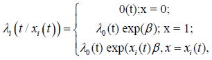
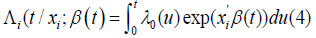
The survival models exclusively with fixed covariates overtime are widely common and employed in different disciplines. However, the large families of proportional hazards model by nature can be extended to allow for time-varying covariates. Let X(t) denote the value of a vector of covariates for individual i at a time. Then, the extended proportional hazards model is

The multiplicative effect of covariates cannot be separated from time in the clear and easy way and due to the high collinearity with time it is difficult to identify the effects.

To maintain the ideas, we can have the following formulation

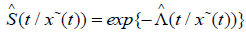
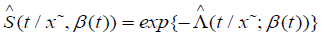
As it was done in above subsection, the survival function can be defined as

However, the problem is when we try to factor out the3 multiplicative effect of cumulative hazard with timevarying covariates from the integral. Unlike it was done in (4), the term multiplicative effect

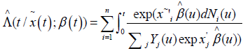
cannot be integrated out from (6). Therefore, the empirical cumulative hazard estimator of (6) can be derived in more complex way than the one in (4) and is given below as

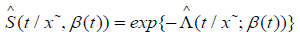
Similarly, the corresponding estimated survival function can be derived directly from estimated cumulative hazard function as

But, one thing that should be known is unlike in case of time invariant covariates, the estimated survival function cannot be simplified in to . A unique integration is need to estimate the consistent estimator for every entire values of rather than multiplication of scalar

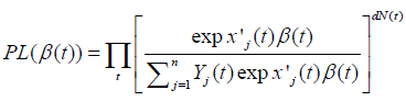
Since the estimation of unknown parameter is always need, we need to think about the usual partial likelihood function. The partial likelihood function for time- dependent covariates is straight forwarding from the Partial likelihood of 1 and we apply the counting process as

In both cases i.e.; in (3) and (5), the model was involved in the proportionality assumption of constant covariate effects of Cox model. However, Cox model can also be extended in to coefficient varying effect model as it will be explained in the next subsection.

Time-Varying Effect

More generally, the survival models can also be extended to allow for time-dependent effects through over time. This extension lead to the lack of proportionality assumptions i.e.; no longer proportionality assumption in the survival models. Thus, the proportional hazard model with the time-varying effect is written as

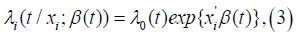
where the parameter β(t) is now a function of time. This model allows for great generality. To maintain the ideas, we can have the following formulation

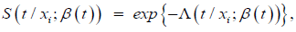
As it was done in above section, the survival function can be defined as

however, the problem is when we try to factor out the multiplicative effect of cumulative hazard with time-varying covariates from the integral; i.e.; it is impossible to get in the form of Unlike it as done in (4), the term multiplicative effect

cannot be integrated out from (6). Therefore, the empirical cumulative hazard estimator of (6) can be derived in more complex way than the one in (4) and is given below as

Similarly, the corresponding estimated survival function can be derived directly from estimated cumulative hazard function as

Thus, one thing that should be known is unlike in case of fixed coefficient effect , the estimated survival function cannot be simplified in to 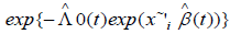. A unique integration is need to estimate the consistent estimator for every entire values of rather than multiplication of scalar

Since the estimation of unknown parameter is always need, we need to think about the usual partial likelihood function. The partial likelihood function for time- dependent covariates is straight forwarding from the Partial likelihood of 1and we apply the counting process as can be shown as

The General Hazard Model

Generally, someone may need to extend this model to more general model that can incorporates both time-varying covariate and time-varying effect. Thus, the combi- nation brings more general version of the hazard model as below.

where x_i(t) is a vector of time-varying covariates referring the realizations of individual subject i at time t, and is a vector of timedependent coefficients, referring the effect that those features have at time t.

The time-dependent effect and time-dependent covariates have been given attentions these days. Finally, the concept of stratifications and frailties which can be applied in all mentioned techniques are other many areas of survival data analysis. The issue of stratified hazard models and frailty hazard models are not included in this report for time being.

As it was done in above section, the survival function can be defined as

however, the problem is when we try to factor out the multiplicative effect 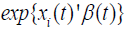of cumulative hazard with time-varying covariates from the integral; i.e.; it is impossible to get in the form of Unlike it was done in (4), the term multiplicative effect

cannot be integrated out from (6). Therefore, the empirical cumulative hazard estimator of (6) can be derived in more complex way than the one in (4) and is given below as

Similarly, the corresponding estimated survival function can be derived directly from estimated cumulative hazard function as

Thus, one thing that should be highlighted is unlike in case of fixed coefficient effect and fixed covariate, the estimated survival function cannot be simplified in to 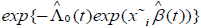. A unique integration is needed to estimate the consistent estimator for every entire values of x˜(t) and β(t) rather than multiplication of scalar .

Since the estimation of unknown parameter is always need, we need to think about the usual partial likelihood function. The partial likelihood function for time- dependent covariates is straight forwarding from the Partial likelihood of 1 and we apply the counting process as can be shown as

Results

Simulation Study

The data is simulated for Cox model in three cases, such as with fixed covariates, with time-varying covariates and time-dependent effects. The data was generated by using sim. survdata() under R package ”coxed” based on the flexible hazard methods described by Harden JJ [2]. The survival time data with two covariates one categorical and one continous was generated with sample size n=500 and maximum duration 60 units using sim. survdata(). By default, sim. survdata() generates the survival time and three covariates from standard normal distribution. However, we can adjust for other characteristics of covariates from different distributions.

A. Procedures: install.packages(”coxed”); library(coxed)

B. Default case: Rdata < −sim.survdata(N = 1000, T = 100, num.data.frame =1)

C. Our case: For fixed covariates and fixed effects : x¹ < − rbinom(500, 1, 0.5); x² < −rnorm(500, 0, 1); z < −data.frame(x¹, x²) Rdata < −sim.survdata(N = 500, X = z, T = 60, num.data. frame = 1) head(R data $data)

Table 1 Illustrates the top features of numerical observations from each variables of the survival data generated by ”sim. survdata()” functions under R library package ”coxed”. Head (R data$ baseline).

Table 2 Illustrates the characteristics of baseline density function, cumulative distribution, survival function, hazard function and cumulative hazard functions of survival time from the defined origin until the event or censor occurs. Rt data <−sim.survdata(N = 500, T = 60, xvars = 2, censor = 0.30, censor.cond = ”TRUE”, num.data. frames = 1).

Table 3 Shows the results of Cox Proportional hazards (PH) model with baseline or fixed covariates. The result has shown statistical insignificance for both covariates (P-value=0.921 and 0.818) respectively.

Simulation for Time-Varying Covariates

Required data structure for time-dependent covariate is technically different from the survival data structure with baseline covariates. The dependent variable for Cox model in survival data can be arranged by using”Surv()” function in survival pack- age of R software. Commonly it has two arguments survival time and a censoring time variables. However, for in the case of time-varying covariates the survival time variable setup is divided in to two sections referring start and end of discrete in- tervals, which in turn permits a covariate to be measured in different values across different intervals for the same observations. Thus, in the case of time dependent co- variates, we set type=”tvc” in ”sim.survdata()” function to generated survival time data with time varying covariates. Then the survival durations are generated again using proportional hazards, and are passed to the ”permalgorithm()” function in the ”permAlgo” package to generate the time-varying data structure [3]. In the case of time-dependent covariates, the type=”tvc” option of sim.survdata does not allow to to use user supplied data for the covariates, as a time-varying covariate is expressed overtime frames which them selves convey part of the variation of the times, and then the time is generated [4]. Rtdata < −sim.survdata(N = 500, T = 60, xvars =2, censor = 0.30, type = ”tvc”, censor.cond = ”TRUE”, num.data.frames = 1).

The results that shown in Table 4 is about the Cox PH model with time-varying covariates and similar to the results of Cox Model in Table 3, the results were found statistically insignificant (P-value=0.708 and 0.450) but relatively better than the results of Cox PH model with baseline covariates.

Simulation for Cox Model with Time-Varying Coefficient

The usual proportionality assumptions of Cox proportional hazard model fail when the coefficient effect varies through overtime. The data for time-dependent coefficients can similarly generated using sim.survdata() function by setting the type=”tvbeta” option inside the function. Whenever this option sets, the first coefficient, whether coefficients are user-supplied or randomly generated, is interacted with natural log of the time counter from 1 to maximum time T [4]. Then the sim.survdata() function generates survival time from proportional hazards model, and saves the coefficients in designed matrix form to allow their dependence on time. So to generate data with time-dependent coefficients set type=”tvbeta” as below.

Rtdata < −sim.survdata(N = 500, T = 60, xvars = 2, censor = 0.30, type = ”tvbeta”, censor.cond = ”TRUE”, num.data.frames = 1)

In Table 5, the result of the Cox PH model with time-varying coefficient and baseline covariates were considered. The results have shown strong statistical signif- icance (P − values < 0.001). This in turn is the indication of non-proportionality in the survival data.

Simulation for General Cox Model with Time-Varying Coefficient and Time-Varying Covariates

The usual proportionality assumptions of Cox proportional hazard model fails when the coefficient effect varies through overtime and also covariates change overtime. The data for general cox model with time-dependent coefficients and time-dependent covariates can similarly generated using sim.survdata() function by setting the type=c(”tv”,”tvbeta”) option inside the function. Whenever this option sets, the first coefficient, whether coefficients are user-supplied or randomly generated, is in- teracted with natural log of the time counter from 1 to maximum time T [4]. However since user-supplied is not applicable for time-varying covariates we just use random generated data instead. Then the sim.survdata() function generates survival time from Cox model, and saves the coefficients in designed matrix form to allow their dependence on time. So to generate data with time-dependent coefficients and time- varying covariates set type=c(”tv”,”tvbeta”) as below.

Rtbdata < −sim.survdata(N = 500, T = 60, xvars = 2, censor = 0.25, type = c(”tvc”, ”tvbeta”), censor.cond = ”TRUE”, num.data.frames = 1)

The results of last model have been displayed in Table 6. According the results of Cox PH model with both time-varying covariates and time-varying coefficients, we can conclude that the statistical significance is much more improved with small P-values. For more details take look in the Tables 3-6.

Discussion

Overall this article generally reviews, the works of 1,2,3,4 and come up we summarized results. The article is more or less methodological focusing particularly, in survival analysis of biostatistics and biomedical researches. The article mainly insisted in the comparison of Cox PH models in different cases. In the first model the article exclusively considers baseline covariate and conduct simulation study. In the second model the article incorporated the time-varying covariate and compared with first model. Despite the existence of improvement in p-values the was no enough evidence for significant improvement. Thus, the timevarying coefficient was considered with baseline covariates and the model was highly significant. Generally, overall findings confirm that, failure of proportionality assumption is big trick in Cox PH model of Cox [1]. The gap was solved relaxing the proportionality assumption by incorporating time-varying coefficient in the Cox model. Consistent to the findings of 4, our findings explicitly have shown high significance in results in the case of considering timevarying covariate in the Cox PH model.

Likewise, even though it was not perfect unlike the result of 3 in their simulation studying with the consideration of time-varying covariates, our results have shown reasonable improvement when the time-varying covariates are considered. More ad- vanced approach related to this article is employed by Fissuh et al. [5] under semiparametric transformation models. Their recently published paper shows the im- portance of time-varying covariate and time-varying coefficient effects in advanced survival models.

Conclusion

The article is basically concerned on comparisons of the Cox model with and without the efect of time on covariates and coefficients. The summary review of other works was done, and the result of simulation was included to come up with reasonable review of the article. The data were generated in four different cases under the” sim.survdata()” function of R package called ”coxed”. Then the results of four models were compared based on the simulation result. The result has shown that the last model in which both time-dependent covariates and time-dependent coefficients considered was relatively better performed than the rest models with small standard errors and P-values of significance. Therefore, we can give the general conclusion that when the proportionality assumption of Cox model fail to fulfill, incorporating the timevarying coefficient effect in the model is advisable. The considering baseline covariate may not be always true because there is the time when the covariate changes overtime. Thus, incorporating time-varying covariate in the model may help us to get reasonable results. Some- times it can be happened that both covariate and coefficient effect changes overtime. Thus, incorporating both timevarying covariates and time-varying coefficients shall give us more reasonable results.

In this article the widely applicable right censoring was considered. However, extending to other censoring mechanism can be the further work of this article. The other further work of this article can be extended to consider the truncation time in the model. In this article the details about the large sample theories and counting process techniques were not much employed explicitly. Thus, deriving the consistency of the unknown parameters using large sample properties is more advisable. Counting process is the attractive part of the survival data analysis that could provide us reasonable results.

Declaration

This study never considered anything related to the ethical approval and consents. The study was totally free of any unethical participation. We can certify that there was no anything related to animals or human being particularly children related researches. Unfortunately, this article was not funded by any funder because the work has done by the personal motivation and has not submitted to any organization or institute. The work was done for personal promotion and may help the authors for academic promotion in future. Therefore, the consent for publication was for dual purpose. The first purpose is to contribute the professional skill in the scientific research of the academics for the readers and beginning researchers. The second purpose is for personal academic promotion of the authors.

We declare this article is a result of our genuine contribution and all sources of materials used for literature have been duly acknowledged. There was no competing interest in this article. All authors contributed to write this article and have no interest of conflict among. The work was mainly done by the first and corresponding author with high contribution. However, the contributions of second, third, fourth and fifth authors were constructive to improve the quality of the article all authors contribute for the grammatical correction. The fourth author as expert of computer science, contributed in consulting simulation study and the second author as a mathematician contributed in consulting mathematical equations. Overall the contribution of all authors except first author were equivalent and should considered as the equivalent contributors. Generally, more than 75% of the work has been done by the corresponding author.

References

1. Cox DR (1972) Regression Models and Lifetables, Springer New York. pp. 527-541.
2. Harden JJ, Kropko J (2018) Simulating duration data for the cox model. Political Science research and Methods 2018. 18.
3. Sylvestre MP (2008) Comparison of algorithms to generate event times conditional on time-dependent covariates. Statistics in Medicine 27(14): 2618-2634.
4. Kropko J, Harden JJ (2018) How to simulate survival data with the sim. survdata function.
5. Fissuh YH, Woldu TG, Ahmed IAI, Kebebe AZA (2019) Simulation Study on Comparing General Class of Semiparametric Transformation Models for Survival Outcome with Time-Varying Coefficients and Covariates. Open Journal of Statistics 9(2): 169-180.