


Lupine Publishers Group
Lupine Publishers
ISSN: 2644-1381
Review Article(ISSN: 2644-1381) 
A Note on Relative Potency Theorem Volume 3 - Issue 5
Received: September 21, 2022 Published: October 07, 2022
*Corresponding author: Ogoke Uchenna Petronilla, University of Port Harcourt, Nigeria
DOI: 10.32474/CTBB.2022.03.000171
Abstract
In this work, further relative potency properties and a thorough proof have been attained. The findings are derived using the Taylor’s (Maclaurin’s) series, and the expected value and variance of the relative potency are as a consequence. Alternately, the first and second moment for the relative potency (R)are obtained given the potency.
Introduction
The common assumption is that the test doses and the standard doses have the same variance and follow two normal distributions (Bivariate Normal Distribution) [1]. Suppose we have {XT1, XT2, XT3… XnT} which are identical and independently distributed N() and {XS1, XS3, XS3, ... , XnS } are also identical and independently distributed and N(), where ρ = μS/μT is estimated by

where: ns is the number of subjects assigned to the standard preparation
nT is the number of subjects assigned to the test preparation.
XSi is the Individual Effect Dose (IED) of the ith subject receiving the standard preparation.
XTj is the IED of the jth subject receiving the test preparation.
The proof and other properties (first and second moments) have not been fully explained in the literature. Hence the need to address these.
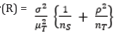
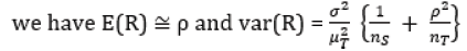
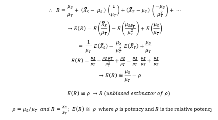
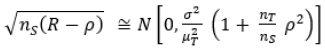
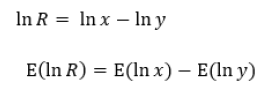
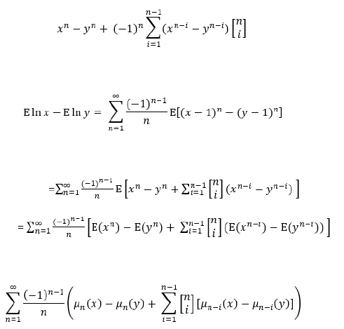
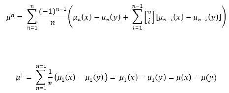
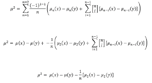
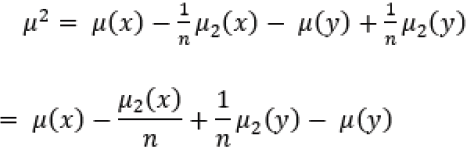
Proof: Let {XSi : i = 1, …, ns} be a random sample from a population (not necessarily normal) with mean and variance while {XTi : i = 1, …, nT} is a random sample from a population (not necessarily normal) with mean and variance where the samples are independent. Then if and ρ = /, we have E(R) ρ and var
Note: R is a ratio of two random variables and so its expected value is not
Note: R is a ratio of two random variables and so its expected value is not
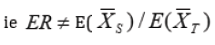
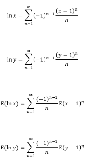
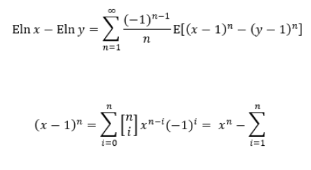
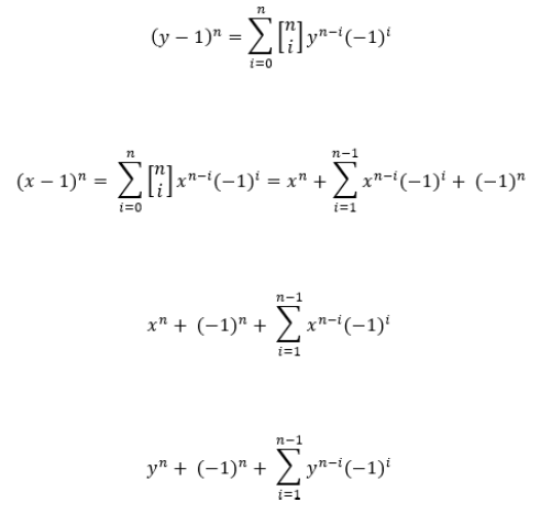
Proof: The following results can be derived from the Taylor’s (Maclaurin’s) series.
If f(x,y) = f(a,b) + (x − a) + (y ̶ b) + ... (1)
where expansion is about x = a and y = b.
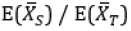
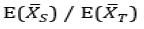
Let R = relative potency of the sample
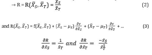
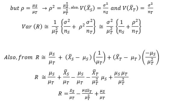
Corollary : Given that the populations in the Theorem above is normal, then
Remark
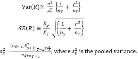
a. Homogeneity of Variance: For ease of comparison, the variance of the two preparations is assumed to be equal. To test this assumption, we use the F-distribution, where nS – 1 is the numerator degree of freedom and nT – 1 is the denominator degree of freedom [2].
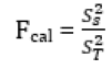
where and are the sample variances of the standard and test preparations respectively.
b. Variance Estimate: Following from Theorem above,
Establishing the Moment Generating Function for the relative potency, R.
Given

where
Conclusion
A detailed proof and other properties of relative potency have been established, hence, certain other expression; the coefficient of variation, skewness and kurtosis can be obtained [3].
References


-

Mark E Smith
Bio chemistry
University of Texas Medical Branch, USA -

Lawrence A Presley
Department of Criminal Justice
Liberty University, USA -

Thomas W Miller
Department of Psychiatry
University of Kentucky, USA -

Gjumrakch Aliev
Department of Medicine
Gally International Biomedical Research & Consulting LLC, USA -

Christopher Bryant
Department of Urbanisation and Agricultural
Montreal university, USA -

Robert William Frare
Oral & Maxillofacial Pathology
New York University, USA -

Rudolph Modesto Navari
Gastroenterology and Hepatology
University of Alabama, UK -

Andrew Hague
Department of Medicine
Universities of Bradford, UK -

George Gregory Buttigieg
Maltese College of Obstetrics and Gynaecology, Europe -

Chen-Hsiung Yeh
Oncology
Circulogene Theranostics, England -
.png)
Emilio Bucio-Carrillo
Radiation Chemistry
National University of Mexico, USA -
.jpg)
Casey J Grenier
Analytical Chemistry
Wentworth Institute of Technology, USA -

Hany Atalah
Minimally Invasive Surgery
Mercer University school of Medicine, USA -

Abu-Hussein Muhamad
Pediatric Dentistry
University of Athens , Greece
