


Lupine Publishers Group
Lupine Publishers
ISSN: 2637-4579
Research Article(ISSN: 2637-4579) 
A Comprehensive Study on EMG Feature Extraction and Classifiers Volume 1 - Issue 1
Received: January 25, 2018; Published: February 07,2018
Corresponding author: Christopher Spiewak, Milwaukee, Mechanical Engineering Department, University of Wisconsin-Milwaukee, USA, Email: cspiewak@uwm.edu
DOI: 10.32474/OAJBEB.2018.01.000104
Also view in:


Abstract
In the past few years the utilization of biological signals as a method of interface with a robotic device has become increasingly more prominent. With the many of these systems being based on EEG and EMG.EMG based control has five main parts data acquisition, signal conditioning, feature extraction, classification, and control. This paper seeks to briefly cover the aspects of data acquisition and signal conditioning. After which, various methods of feature extraction, and classification are discussed.
Introduction
The use of EMG in Brain-Computer Interaction (BCI) as part of a Human-Computer Interface (HCI) is a method of control that allows for a more natural use of one's own existing muscles. Electromyography (EMG) is measured from the muscles as they receive the signal of activation from the brain. This paper presents an analysis of various methods of feature extraction and classification of the EMG signals. As EMG rapidly fluctuates with time and can contain some corruption in the data, due to noise. This means it is critical to choose the methods of feature extraction and classification to improve accuracy and to decrease the computational demand.
The methodology of EMG based control is mainly concerned with data acquisition, signal conditioning, feature extraction, classification, and then control (Figure 1) [1]. This paper presents in the next section a brief description of the method of data acquisition. Then following this will also be a brief description of signal conditioning. Next, the methods of feature extraction are presented. Each method is described with an equation and is then experimental results are presented for easy comparison. All the simulations were done in MATLAB with scripts all using the same sample size, and segment length. The following section then goes on to present different methods of classification in their formal nature. This paper then concludes with a discussion of the pros and cons of the different methods of feature extraction techniques and some specific application of those techniques. As well as a discussion of the different classifiers and some possible specific application of those classifiers.
Figure 1: Block diagram of the process of EMG processing for control.

Data Acquisition
EMG data can be gathered in two different ways: invasive, and noninvasive [2]. The invasive method is performed by inserting a needle type electrode through the skin into the muscle desired. This technique is mostly used for diagnostic purposes. The invasive method provides high-resolution data, and accurate localized descriptions of muscle activity. This method, however, does cause some discomfort to the patient, and is not suited for repeated daily use. The noninvasive method uses surface mounted electrodes commonly positioned over specific muscles. This decreases the patient s discomfort and allows for the ability to be a fully portable device. The accuracy and resolution of the device depends on the sampling rate and the segment length [3]. This method has commonly used adhesives and conductive gels for the mounting of the electrodes. However, in recent years the improvement of surface mounted EMG sensors has made it possible to mount sensors without adhesive or gel.
Signal Conditioning
Data segmentation is done using two main methods: overlapping segmentation, and disjoint segmentation [4]. Disjoint segmentation uses separate segments with predefined length for feature extraction (Figure 2). While in overlapped segmentation, the new segment slides over the current segment, where the interval of time between two consecutive segments is less than the segment length and more than the processing time (Figure 3). This shows that disjoint segmentation of data is associated with segment length. While overlapped segmentation of data is associated with segment length and increment [5]. In experiments done by Oskoei, and Hu [4], disjoint and overlapped segmentation was compared to display their classification performance. The length of 50ms was used in disjoint segments whereas overlapped systems used segments having a length of 200ms with an increment of 50ms. The results showed that the defined disjoint segmentation 200ms provided high performance in EMG classification and an adequate response time allowing for real-time use. With the defined overlapped segmentation shortening the response time without noticeably degrading the accuracy of data. This indicates that to maintain an efficient use of computational resources while not compromising the accuracy of data, it is imperative to implement an appropriately timed method of overlapped segmentation.
Figure 2: Graphical representation of disjoint segmentation [4].

Figure 3: Graphical representation of overlapping segmentation [4].

Feature Extraction
Feature extraction is the transformation of the raw signal data into a relevant data structure by removing noise, and highlighting the important data. There are three main categories of features important for the operation of an EMG based control system. Those being the time domain, frequency domain, and the time-frequency domain [1,5]. However, due to the intense computation needs of transformations required by the features in the time-frequency domain, this method is not used for therapeutic devices.
Time Domain
Features in the time domain are more commonly used for EMG pattern recognition. This is because they are easy, and quick to calculate as they do not require any transformation. Time domain features are computed based upon the input signals amplitude. The resultant values give a measure of the waveform amplitude, frequency, and duration with some limitations [6]. The methods of integrated EMG, mean absolute value, mean absolute value slope, Simple Square integral, variance of EMG, root mean square, and waveform length will be discussed in more detail in the following sub-sections. Each consecutive section will reuse the same notation for better understanding. For each method, a simple test was done with MATLAB scripts for sake of comparison.
Integrated EMG (IEMG)
Integrated EMG (IEMG) is generally used as a pre-activation index for muscle activity. It is the area under the curve of the rectified EMG signal. IEMG can be simplified and expressed as the summation of the absolute values of the EMG amplitude [7]. The filtered results of a simple input can be seen in Figure 4.
Figure 4: IEMG simulation results (raw signal on the left, filtered signal on the right).

Where N is the length of the segment is, i is the segment increment, and xi is the value of the signal amplitude.
Mean Absolute Value (MAV)
The Mean Absolute Value (MAV) is a method of detecting and gauging muscle contraction levels. It is expressed as the moving average of the full-wave rectified EMG signal [7,8]. The filtered results of a simple input can be seen in Figure 5.
Figure 5: MAV simulation results (raw signal on the left, filtered signal on the right).

Mean Absolute Value Slope (MAVS)
The Mean Absolute Value Slope is the estimation of the difference between the MAVs of the adjacent segments. The filtered results of a simple input can be seen in Figure 6. This is expressed as [7]
MAVSi= MAVi+l - MAV (3)
Simple Square Integral (SSI)
The Simple Square Integral (SSI) expresses the energy of the EMG signal as a useable feature [7]. The filtered results of a simple input can be seen in Figure 7.

Figure 6: MAVS simulation results (raw signal on the left, filtered signal on the right).

Figure 7: SSI simulation results (raw signal on the left, filtered signal on the right).

Variance of EMG (VAR)
The Variance of EMG (VAR) expresses the power of the EMG signal as a useable feature. The filtered results of a simple input can be seen in Figure 8. This is defined as [6,7]:
Root Mean Square (RMS)
The Root Mean Square (RMS) is modelled as the amplitude modulated Gaussian random process where the RMS is related to the constant force, and the non-fatiguing contractions ofthe muscles [7]. The RMS method of feature extraction is very commonly used. As it is computationally efficient and quick, while still containing precipice data. The filtered results of a simple input can be seen in Figure 9.
Figure 8: VAR simulation results (raw signal on the left, filtered signal on the right).

Figure 9: RMS simulation results (raw signal on the left, filtered signal on the right).

Waveform Length (WL)
The Waveform Length (WL) is intuitively the cumulative length of the waveform over the segment. The resultant values of the WL calculation indicate a measure of the waveform amplitude, frequency, and duration [7]. The filtered results of a simple input can be seen in Figure 10.
Figure 10: WL simulation results (raw signal on the left, filtered signal on the right).

Frequency Domain
The features extracted using the frequency domains are normally based on a signal's estimated power spectral density (PSD). Except for the Modified Median Frequency and Modified Mean Frequency methods proposed by Phinyomark et al. where the inputs to the methods are the amplitude at the bin frequencies. The frequency domain features in comparison to the time domain features tend to require more computational resources, and time [6]. For each method, a simple test was done with MATLAB scripts for sake of comparison except. As the autoregressive method has many orders of models it has not been simulated for simplicity.
Autoregressive Coefficients (AR)
The Autoregressive (AR) model is a description of each sample of the EMG signal as a linear combination of the previous samples plus a white noise error term. AR coefficients are commonly used as features in pattern recognition [7,9].

Where Xn a sample of the model signal is, ai is the AR coefficients, wn is the white noise error term, and P is the order of the AR model.
Frequency Median (FMD)
The Frequency Median (FMD) is based on the power spectral density (PSD). In general, there are two main types of PSD estimation to calculate the frequency domain feature for EMG: parametric or nonparametric. Parametric methods assume that the signal can be modeled as an output of a linear system. The nonparametric methods do not make any assumptions toward any model of the system. One of the more commonly used methods is the periodogram method [10]. FMD is found as the frequency where the spectrum is divided into two equal parts [7]. The filtered results of a simple input can be seen in Figure 11.
Figure 11: FMD simulation results (raw signal on the left, filtered signal on the right).

Where M is the length of the power spectral density, and (PSD)_ i^th line of the PSD.
The Frequency Mean (FMN) is the average of the frequency. FMN is expressed as the summation of the product of the PSD and the frequency of the spectrum, f_i [7]. The filtered results of a is the simple input can be seen in Figure 12.
Figure 12: FMN simulation results (raw signal on the left, filtered signal on the right).

Modified Median Frequency (MMDF)
The Modified Median Frequency (MMDF) is very similar to the FMD method but is based on the amplitude spectrum, not the PSD. It is an expression of the frequency where spectrum is divided into two regions with equal amplitude [7]. The filtered results of a simple input can be seen in Figure 13.
Where A_j is the EMG amplitude spectrum at the frequency bin j.
Figure 13: MMDF simulation results (raw signal on the left, filtered signal on the right).

Modified Frequency Mean (MMNF)
The Modified Frequency Mean (MMNF) is the average of the frequency based on the amplitude spectrum unlike the FMN [7]. The filtered results of a simple input can be seen in Figure 14.
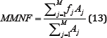
Where fj is the frequency of the spectrum at the frequency bin j and is found similarly to fi.
Figure 14: MMNF simulation results (raw signal on the left, filtered signal on the right).

Classification
Table 1: Classifier Usage.

After the desired features are extracted from the input signal acquired it is the necessary to differentiate the categories amongst the features by using a classifier [11-18]. There are many different types of classifiers to use (Table 1). This study focused on some of the more common methods. Such as neural networks (NN), fuzzy logic (FL), Bayesian classifiers (BC), support vector machines (SVM), linear discriminate analysis (LDA), and neuro- fuzzy hybridization (NF). Multilayer Perceptron (MLP), Fuzzy Min Maxed Neural Network (FMMNN), Hidden Markov Model (HMM), Back-propagation Neural Network (BPN), Log-Linearized Gaussian Mixture Network (LLGMN), Probabilistic Neural Network (PNN), Radial Basis Function Artificial Neural Network (RBFNN), Double-Threshold Detection (DTD), Wavelet Transformation (WT), Wigner-Ville Distribution (WVD), Choi-Williams Method (CWM), Higher-Order Statistics (HOS).
Neural Network (NN)
A Neural Network (NN) refers to; in this case, a supervised learning model meaning that data needs to be labeled before it is processed. The goal of a NN is to imitate a biological brain and its immense network of neurons. This is done by utilizing many simply connected nodes that are weighted. These weights are what the NN uses in its calculations. NNs also have algorithms for learning or training which are used to adjust the weights [19]. ANN has three different classes of nodes: input, hidden, and output nodes (Figure 15). With each class of node organized into a layer where the nodes of the same layer have no connections between each other. There can only be one input, and one output layer. However, there can be any number of hidden layers, as well as any number of nodes with in all layers. The input nodes receive an activation pattern which is then moved in the forward direction through one or more of the hidden nodes then on to the output nodes. The input activation from the previous nodes going into a node is multiplied by the weights of the links over which it spreads. All input activation is then summed and the node becomes activated only if the incoming result is above the node's threshold [20].
Figure 15: Representation of a two layer NN, with one hidden layer and one output layer. Figure by Colin M.L. Burnett used under CC BY-SA 3.0.

Though NNs are a powerful computation model it does not come without a few difficulties. One issue with NNs is that they need to be trained sufficiently to be able to give accurate and precise. During the training, the model needs to be monitored so to not create an over fit or under fit NN. NNs are very good at modeling large datasets with nonlinear features. However, the classification boundaries are difficult to understand intuitively. NNs are also rather taxing computationally and tend to need rather large lookup tables, requiring a large amount of storage space. Though NNs can be trained to solve complex classification problems they cannot use datasets with missing data entries.
Fuzzy Logic (FL)
Fuzzy logic (FL) being a form of multi-valued logic where the logic values possible are in a range of real numbers between 0 and 1. Making FL a mathematical model capable of incorporating and weighing precision and significance. This is done by using the processes of fuzzification, and defuzzification. Fuzzification in a FL system is the process of assigning fuzzy values to the crisp inputs. This is done by choosing an arbitrary curve to represent the relationship between the crisp values and the degree of membership that those inputs contain [21]. This is a fuzzy set, and can be expressed as:
A{ x,μA(x)|x∈U {(14)
Where A is the fuzzy set, U is the universe of discourse with elementsx, and n_A defines the membership function. These fuzzy sets are then tested with a series of if-then statements using logic operators to resolve the output. These results then go through the process of defuzzification to change the fuzzy values back into crisp values. This is done by using numerous different methods such as the centroid, or bisector defuzzification methods. One of the greatest advantages of using FL for classification is that it is flexible, and can be easily modified or combined with several other classification methods. However, FL is not without its drawbacks. FL has many localized parameters and training method. This can make the initial construction, and tuning is very time consuming [22].
Bayesian Classifier (BC)
A Bayesian Classifier (BC) is based on the idea that if a system knows the class it is able to predict the values of the features. Also, if the class is unknown the system can employ Bayes’ rule to predict the class with the given features. Using a BC, the system builds a probabilistic model of the features to predict classes of new instances [23]. Bayes' rule can then be expressed as:
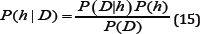
Where P(D|h) is the probability that the training data, D, holds the hypothesis, h; P(h) is the initial probability that is held by the hypothesis; P(D) is the probability that the training data will be observed; P(h|D) is the posterior probability, reflecting the confidence that the hypothesis after the training data has been observed [23,24]. A rather large disadvantage of a BC is that it makes a strong assumption as to the shape of the data distribution. This assumption is that any two features are independent given the output class. This is why BCs are often referred to as a "naive” classifier. However, BCs return with each prediction a degree of certainty. This can be very useful, particularly so when using a method of classifier combination.
Support Vector Machine (SVM)
The goal of a Support Vector Machine (SVM) is to find a hyper plane that corresponds to the largest possible margin between the data points of different classes. To fit the nonlinearity of an EMG signal more appropriately we need to form the SVM to best obtain a quadratic programming (QP) problem. The solution to which will be universal and unique [4]. This can be done by mapping the input data to a richer feature space including nonlinear features. Then the hyper plane is constructed in that space so that all other equations are the same. An advantage of SVM's is that they can use a kernel to decrease the computational strain of higher dimensionality of the mapping function. A kernelis chosen dependent on the application of the SVM. Most kernel algorithms are based on convex optimization or eigen problems which make them statistically well-founded. However, a straightforward SVM's cannot return probabilistic confidence which could be quite helpful depending on the application.
Linear Discriminant Analysis (LDA)
Linear Discriminant Analysis (LDA) is a well-recognized method of feature extraction and dimensionality reduction. LDA is commonly used for dimensionality reduction for pattern recognition, and classification. The goal of LDA is to project a dataset from a high-dimensional space into a lower-dimensional space with class-separability to avoid over fitting, and to improve the tax on the computational resource [25]. This minimizing the within class distance (i.e. precise data clusters) and concurrently maximizing the margin between the classes, thereby achieving the maximum discrimination. This transformation is computed by using the Eigen-decomposition on the scatter matrices from a set of training data [26]. A limitation of LDA is that it is a parametric method as it assumes that the distributions are Gaussian in nature. This will cause the classifier to be unable to preserve any complex structure of data. The biggest complication with using LDA as a classifier is that most if not all the limitations depend on the application.
Neuro-Fuzzy Hybridization (NF)
Neuro-fuzzy hybridization (NF) is the product of the methods of FL and NN leading to the creation of a hybrid intelligent system. This gives the NF system the human-like reasoning style of FL and the learning and connectionist structure of NN. In general, a NF system is based on an underlying FL system and is trained by a data-driven learning method derived from NN theory. The heuristic only takes into account local data to cause local changes in the fundamental FL system. The NF system can be represented as a set of fuzzy rules throughout the learning process. This makes it possible to initialize the NF classifier with or without apriori knowledge [27]. The advantage of using a NF classifier is that it combines the advantages of both FL and NN, human-like reasoning and learning capability. While it also diminishes the disadvantages of both FL and NN, based on apriori knowledge and computationally intensive.
Combination of Classifiers
There has also been research into combination methods of multiple different classifiers. Such as the basis of the NF classifier, which combines the FL and NN methods to overcome the individual methods limitations. This method of combination called Boosting [28]. Boosting is the combination of multiple weak classifiers to create a stronger classifier [29]. Boosting typically helps to reduce the bias, and variance of supervised learning methods [30]. Another method is called voting which is where multiple classifiers are used simultaneously. Each assigning the input to a class, with the final class being the majority voted class [28].There is also a method which presents like a modified version of Voting, called Stacking. Stacking uses multiple classifiers to give input to a meta-classifier which makes the final decision [31].
Discussion
The process of selecting a method of feature extraction is very subjective as there is no generic feature extraction method. However, as seen in section 4.1 many of the time domain based methods display similarly shaped results. Methods based in the time domain are used as an onset index for muscle activity with slight differences in output parameters in each method. The MAVS method gives an output that is quite simplified in nature, smoothing a good portion of the noise in the signal. The RMS method weighs both sides of the raw EMG signal giving a better depiction of the symmetrical fluctuations seen in constant force contractions. Methods based in the frequency domain are generally used for determining muscle fatigue and motor unit recruitment [32-35]. The calculation of motor unit recruitment is an important parameter as it exhibits the increasing strength of a voluntary contraction. Which more appropriately displays the nonlinear nature of muscle expansion and contraction? In this paper, we also presented six different methods of classification. Each having slight differences in their strengths and weaknesses. Highlighting the importance of evaluating the method of classification to more appropriately fit the application.
References
- Zecca M, Micera S, Carrozza MC, Dario P (2002) Control of multifunctional prosthetic hands by processing the electromyographic signal. Critical Reviews in Biomedical Engineering 30(4-6): 459-485.
- Sörnmo L, Laguna P (2005) Bioelectrical signal processing in cardiac and neurological applications. Academic Press, Biomedical Engineering8.
- Al-Mulla MR, Sepulveda F, Colley M (2011) A Review of Non-Invasive Techniques to Detect and Predict. Sensors(Basel) 11(4): 3545-3594.
- Oskoei MA, Hu H (2008) Support vector machine-based classification scheme for myoelectric control applied to upper limb. IEEE transactions on biomedical engineering 55(8): 1956-1965.
- Rechy-Ramirez EJ, Hu H (2011) Stages for Developing Control Systems using EMG and EEG signals: A survey. School of Computer Science and Electronic Engineering, University of Essex pp. 1744-8050.
- Oskoei MA, Hu H (2006) GA-based feature subset selection for myoelectric classification. IEEE International Conference on Robotics and Biomimetics, Kunming, China.
- Veer K, Sharma T (2016) A novel feature extraction for robust EMG pattern recognition. Journal of medical engineering & technology 40(4): 149-154.
- Alkan A, Gunay M (2012) Identification of EMG signals using discriminant analysis and SVM classifier. Expert Systems with Applications 39(1): 4447.
- Cesqui B, Tropea P, Micera S, Krebs HI (2013) EMG-based pattern recognition approach in post stroke robot-aided rehabilitation: a feasibility study. Journal of neuroengineering and rehabilitation 10(1): 75.
- Zhang ZG, Liu HT, Chan SC, Luk KDK, Hu Y (2010) Time-dependent power spectral density estimation of surface electromyography during isometric muscle contraction: Methods and comparisons. Journal of Electromyography and Kinesiology 20(1): 89-101.
- Choi C, Micera S, Carpaneto J, Kim J (2009) Development and quantitative performance evaluation of a noninvasive EMG computer interface. IEEE Transactions on Biomedical Engineering 56(1): 188-197.
- Han JS, Song WK, Kim JS, Bang WC, Heyoung L, Zeungnam B (2000) New EMG pattern recognition based on soft computing techniques and its application to control of a rehabilitation robotic arm. Proc of 6th International Conference on Soft Computing (IIZUKA2000).
- Hussein SE, Granat MH (2002) Intention detection using a neuro-fuzzy EMG classifier. IEEE Engineering in Medicine and Biology Magazine 21(6): 123-129.
- Ahsan MR, Ibrahimy MI, Khalifa OO (2011) Hand motion detection from EMG signals by using ANN based classifier for human computer interaction. 4th International Conference on Modeling, Simulation and Applied Optimization (ICMSAO).
- Bu N, Okamoto M, Tsuji T (2009) A hybrid motion classification approach for EMG-based human-robot interfaces using bayesian and neural networks. IEEE Transactions on Robotics 25(3): 502-511.
- Ahsan MR, Ibrahimy MI, Khalifa OO (2009) EMG Signal Classification for Human Computer Interaction: A Review. European Journal of Scientific Research 33(3): 480-501.
- Reaz MBI, Hussian MS, Mohd-Yasin F (2006) Techniques of EMG signal analysis: detection, processing, classification and applications. Biological procedures online 8(1): 11-35.
- Micera S, Sabatini AM, Dario P, Rossi B (1999) A hybrid approach to EMG pattern analysis for classification of arm movements using statistical and fuzzy techniques. Medical engineering & physics 21(5): 303-311.
- Krõse B, van der Smagt P (1996) An Introduction to Neural Network, Amsterdam, Netherlands: University of Amsterdam.
- Ferreira C (2006) Designing neural networks using gene expression programming. Applied soft computing technologies: The challenge of complexity, Springer-Verlag Berlin Heidelberg pp. 517-535.
- Novák V, Perfilieva I, Mockor J (2012) Mathematical principles of fuzzy logic. Springer Science & Business Media.
- Albertos P, Sala A (1998) Fuzzy logic controllers. Advantages and drawbacks. VIII International Congress of Automatic Control.
- Poole DL, Mackworth AK (2010) Artificial Intelligence: foundations of computational agents. Cambridge University Press, USA.
- Mitchell TM (1997) Machine Learning, McGraw-Hill Education, USA.
- Raschka S (2014) Linear Discriminant Analysis - Bit by Bit.
- Phinyomark A, Hu H, Phukpattaranont P, Limsakul C (2012) Application of Linear Discriminant Analysis in Dimension. Measurement Science Review 12(3): 82-89.
- Buckley JJ, Hayashi Y (1994) Fuzzy neural networks: A survey. Fuzzy Sets and Systems 66(1): 1-13.
- Lotte F, Congedo M, Lecuyer A, Lamarche F, Arnaldi B (2007) A review of classification algorithms for EEG-based brain-computer interfaces. Journal of neural engineering 4(2): R1-R13.
- Zhou ZH (2012) Ensemble methods: foundations and algorithms, CRC Press, USA.
- Breiman L (1996) Bias, Variance, and arcing classifiers. University of California-Berkeley, Berkeley, CA.
- Wolpert DH (1992) Stacked generalization. Neural networks 5(2): 241259.
- Oskoei MA, Hu H, Gan JQ (2008) Manifestation of fatigue in myoelectric signals of dynamic contractions produced during playing PC games. 30th Annual International Conference of the IEEE pp. 315-318.
- Volpe BT, Krebs HI, Hogan N (2001) Is robot-aided sensorimotor training in stroke rehabilitation a realistic option? Current opinion in neurology 14(6): 745-752.
- Prange GB, Jannink MJ, Groothuis-Oudshoorn CG, Hermens HJ, IJzerman MJ (2006) Systematic review of the effect of robot-aided therapy on recovery of the hemiparetic arm after stroke. Journal of rehabilitation research and development 43(2): 171-184.
- Kiguchi K, Tanaka T, Fukuda T (2004) Neuro-fuzzy control of a robotic exoskeleton with EMG signals. IEEE Transactions on fuzzy systems 12(4): 481-490.

Editorial Manager:
Email:
biomedicalengineering@lupinepublishers.com

-

Mark E Smith
Bio chemistry
University of Texas Medical Branch, USA -

Lawrence A Presley
Department of Criminal Justice
Liberty University, USA -

Thomas W Miller
Department of Psychiatry
University of Kentucky, USA -

Gjumrakch Aliev
Department of Medicine
Gally International Biomedical Research & Consulting LLC, USA -

Christopher Bryant
Department of Urbanisation and Agricultural
Montreal university, USA -

Robert William Frare
Oral & Maxillofacial Pathology
New York University, USA -

Rudolph Modesto Navari
Gastroenterology and Hepatology
University of Alabama, UK -

Andrew Hague
Department of Medicine
Universities of Bradford, UK -

George Gregory Buttigieg
Maltese College of Obstetrics and Gynaecology, Europe -

Chen-Hsiung Yeh
Oncology
Circulogene Theranostics, England -
.png)
Emilio Bucio-Carrillo
Radiation Chemistry
National University of Mexico, USA -
.jpg)
Casey J Grenier
Analytical Chemistry
Wentworth Institute of Technology, USA -

Hany Atalah
Minimally Invasive Surgery
Mercer University school of Medicine, USA -

Abu-Hussein Muhamad
Pediatric Dentistry
University of Athens , Greece
