On Hydrogeological Calculation of Pressure Redistribution in the Artesian Aquifer in Case of Abrupt Reduction of Water Intake Volume 10 - Issue 2

NG Aloyan*

• National Agrarian University of Armenia, Armenia

Received: September 23, 2022;   Published: September 30, 2022

Corresponding author: National Agrarian University of Armenia, Armenia

DOI: 10.32474/CIACR.2022.10.000331

Abstract PDF

Abstract

A hydrogeological calculation method is given to determine the partial restoration of the piezometric pressure in the artesian aquifer when the flow rate of the fountain pumping water from there is abrupt reduced at some point in time. During the development of the calculation method, it was assumed that at the same time with the fountain well, in the same place, an injecting vertical well would start operating, the flow rate of which would be equal to that reduced size. It is also accepted that although the edge condition on a fountain well is non-linear, the principle of superposition applies here. The computational method test based on the results of network model studies gave sufficient accuracy (the average deviation was about 4%).

Keywords: Artesian aquifer; piezometric pressure; fountain well; abrupt reduction of flow rate; injecting well; superposition

Introduction

The underground component, the main volumes of which are enclosed in the Artesian Basin of The Ararat Valley (ABAV), differs from the general water resources of the Republic of Armenia by a number of features. The ABAV consists of three aquifers, of which the third is the high-pressure layer, from which water can be drawn through fountain wells using the internal elastic strength of the layer, thus avoiding the use of deep pumps and electricity. After 2000, the construction of fish ponds, for which the waters of that layer were used, began to flourish in the ABAV. Moving only for their own interests, various individual entrepreneurs in the layer with a fiery, chaotic horse, without the appropriate hydrogeological calculations and projects, installed numerous fountain wells, through which they carried out super-normative water intake. In particular, in 2013 only for the needs of fishponds, 35.5 m3/s of water was taken from the pressure aquifer through fountain wells, while the water supply to the layer was officially confirmed at 34.7 m3/s [1]. Due to such water intake, an ecological catastrophic situation has been created in the ABAV, the further existence of these fishponds is under threat of extinction. In order to correct the situation to some extent, the RA government has taken several measures since 2014. 49 wells were dismantled, 41 were conserved, and the flow rates of 225 fountain wells were shut off to the officially permitted level for each. The positive results of the measures taken are already obvious, the outflows of some wells are gradually increasing, the piezometric pressure in the aquifer is increasing. It should be noted that the owners of the fountain wells brought to the valve mode are already using various aeration devices that enrich the pond water with oxygen to reduce the outflows.

Materials and Methods

It is important to calculate, to predict the observed increase in piezometric pressure due to the sharp decrease in water intake, in order to effectively operate the ABAV pressure water supply layer, to gradually improve the disturbed energy condition. The theoretically posed problem is to solve the second degree partial differential equation describing the unconfirmed filtration motion in the elastic water layer when the boundary conditions ensuring the uniformity of the solution are complex. This complication creates the edge condition of the 2nd sex on the fountain well, which is a linear function, and at t> 0 it becomes a ruptured function due to the introduction of additional hydraulic resistance in the well. In addition, the initial condition of the first sex (t = 0), which characterizes the field of piezometric pressures in the aquifer, is a function of the coordinates of the points in the layer. It should be noted that due to some circumstances, the issue was considered not axial symmetry, but planned. The complex appearance of the term conditions does not allow the equation to be solved analytically, so it has been done numerically using the principles of mathematical analogy on network models, as well as the principles of hydraulic modeling.

A time-consuming continuous hydraulic integrator was used, where ordinary distilled water was used as the working material. The methodology of the study of the work of the fountain well installed in the pressure water layer by means of a hydraulic integrator and the technique is described in detail in the work [2]. and here are the final results of the numerical solution of the differential equation of filtration motion for a specific case. The following case was considered. A vertical well with radius r = 0.105 m was installed in its entire depth in the pressure water layer. The conductivity of the layer is T = km = 3000 m²/day, the elastic water supply coefficient μ * = 0.01, the initial positive piezometric pressure is He = 15.0 m. The aquifers are cracked basalts, which eliminates the need to install a filter in the well intake. Therefore, the well can be considered perfect (ξ = 0) according to the size of the passage of the aquifer. The fountain well installed in the layer operates normally for 50 days, after which its flowt is abrupt reduced by means of a valve, introducing additional local hydraulic resistance. Well operation in this new mode is observed for up to 50 days. The fountain well on the hydraulic integrator is modeled according to its total hydraulic resistance, which is determined by the following connection [3].

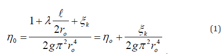
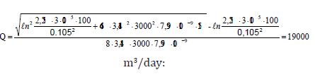
where η_o is the initial hydraulic resistance of the well, ℓ is the depth of the well, r_o is its radius, λ is the coefficient of hydraulic contact of Darcy, ξ_k is the additional local hydraulic resistance introduced by the valve, g is the acceleration of free fall. For the observed well according to formula (1) we get η_o = 7.59 ·10^-9 days²/m⁵. It is modeled on a 3.5 cm long capillary with a diameter of 0.058 cm. By entering the model values of water layer characteristics (filtration resistances) and piezometric pressures in the hydraulic integrator with the well model, an analogous model of the complete “Water layer-fountain well” system is created. Work on the fountain well to = 50 days was observed on this model. The output of the fountain well corresponding to that day was measured (Q = 19200 m3/day) and piezometric pressure drops at individual points of the aquifer. Some of their values are given in line 1 of the table. This data will be a starting point for solving the problem of partial recovery of the pressure we are interested in. That is, for this problem to = 50 days becomes t = 0 condition. Naturally, ξ_k = 2,24 local hydraulic resistance is introduced in the well through the valve, in which case according to (1) the connection will be η = 2,03·10^-8 days²/m⁵. To model it, the length of the capillary becomes 9.5 cm, and the diameter, which provides the condition of the fountain, remains the same. As a result, the well flow rate decreases sharply to 157570 m3/day, which is later changed to insignificant amounts (see table). The process of restoring piezometric pressures takes place in the aquifer, it is observed for a period of 50 days. The value of pressure drops at some characteristic points of the well flow rates and aquifer are given in the (Table 1) below.

The data from the table show that due to the high piezoelectricity of the aquifer, the effect of this change is already observed at a distance of r=1000 m only one day after the reduction of the well outlet, and at a distance of r = 2000 m this effect is already observed after 10 days. The pressure drops at this point continued to increase. It should be noted that a more comprehensive (cascad ing) problem was considered on the hydraulic integrator, when the fountain well flow rate was reduced in non-separate phases (only the data of phase I are given here, and the whole problem will be discussed in our future articles). They give a very positive result quickly; they should be used on ABAV fountain wells. From an economic- ecological point of view, it is possible to identify in advance the fountain wells, the flow rates of which need to be reduced first and to determine the amount of that reduction and regime in order to ensure the necessary pressure restoration at the target points of the aquifer. The answer to this question can currently be given using the modeling method, but it is associated with some technical difficulties and is not operational in terms of time. Therefore, it is more expedient to develop a special calculation method, which will allow determining the amount of partial pressure restoration at different points of the aquifer, depending on the number of times the fountain flow is reduced over the time. First we accept that if at some point in time the flow rate of the fountain well is ebrupt reduced, it is equivalent to the fact that the well continues to operate in its former undisturbed mode, but at the same time from the same point in the same place begins to inject a vertical well with equal flow rate to that reduced size. In the observed example it is ΔQ = 19200-15570 = 3630 m³/day. If the design values of the fountain wells are not included in the calculations, then they can be determined with the following formula by [4].

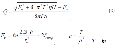
where: T is the conductivity of the layer, a is piezoelectricity, k is the filtration coefficient, m is the strength of the layer, μ * is the coefficient of elastic water supply, r_o is the radius of the well, η is its total hydraulic resistance, ξ_timp is the coefficient of total imperfection, t is the time for which the flow rate is calculated. The second acceptance concerns the joint work of two vertical wells. We accept that the non-linear boundary condition on the fountain well does not preclude the application of the principle of motion (superposition) when making calculations here, since the equation describing the filtration motion in a pressurized water layer is linear. That is, at some point in the aquifer, the final pressure drop will be the algebraic sum of the pressure changes due to the operation of the two wells. In the case of an imaginary injector well, the increase in pressure in the aquifer, as accepted in groundwater dynamics, will be determined by the formula known as Ch. Teys (Only the flow rate changes) [5,6].

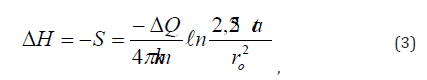
where ΔQ is the injected flow rate, ΔH is the increase in piezometric pressure. In case of working of the well with increasing pressure drops in the water layer, we define with by the following formula of [4].

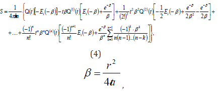
where: r is the distance from the point to the well, Q⁽ⁿ⁾(t) is the n_th order derivative of the flow rate over time, e is the basis of the natural logarithm,

i E is the exponential pointer function. If β <0.05, then without making a big mistake (not more than 5%) can be accepted.

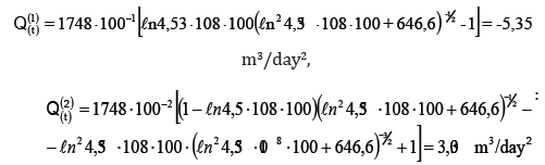
Calculations show that the first three members of the series can be satisfied in Equation (4) without making significant mistakes. In that case Q⁽¹⁾(t) and Q⁽²⁾(t) will be obtained from connection (2) and will have the following forms:

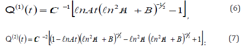
The following appointments are made here:

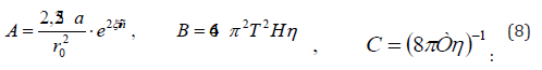
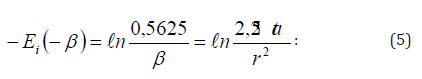
Determine the piezometric pressure drop at the points of the aquifer at distances r₁ = 500 m and r₂ = 1000 m from the well 50 days after the abrupt reduction of the well flow rate. First, with relation (3) determine the pressure recovery at points r1:

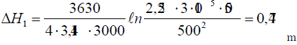
With such a mode at points r₂ we will get ΔH₂ = 0.34 m.

(4) determines the pressure drops at the same points from the fountain well operating t = 100 days after assuming that no additional hydraulic resistance has been introduced. The well flow rate for t = 100 days will be according to formula (2).

Determine the derivatives Q⁽¹⁾(t) and Q⁽²⁾(t) for t=100 days. The values of the appointments will be:

Á = 4,53 ⋅10 ⁸ , B =646.6 , C =1748:

From (6) and (7) we will get respectively:

Determine the pressure drop by Equation (4) when r = 500 m, we will have:

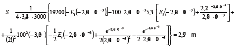
The final drop in pressure at the points 500 m from the aquifer will be:

ΣS = S – ΔH = 2,97- 0,47 = 2,5 m:

As a result of the model study, as seen from the last line of the table, ΣS = 2.38 m, the deviation is 4.8%.

Making such a calculation, when r = 1000 m, we will get: S = 2.14 m, and ΣS = 2.14 - 0.34 = 1.8 m. In the model, the reduction was 1.73 m (deviation - 3.9%).

Conclusion

The change in piezometric pressure in the artesian aquifer can be determined by hydrogeological calculation formulas (3) and (4) under the conditions of abrupt reduction of the flow rate of the wells, which is equal to a reduced extent, as the principle of superposition applies here. When calculating the pressure drop in Equation (4), it is assumed that the fountain well is operating in a non-disrupted mode. The deviation of the computational-model results is within the permissibility limits.

References

1. USAID (2014) Clean Energy and Water Program. Assessment of groundwater resources in the Ararat Valley. Yerevan pp. 77.
2. Melikyan NL (2006) Methods of efficient use and management of exploitable water resources of the artesian basin. Doctoral dissertation, Yerevan 350.
3. Melikyan NL and Aloyan NG (2015) By the method of hydrogeological calculation of the regulated water intake from the high-water aquifer. Journal, "Banber" National Polytechnic University of Armenia, series «Hydrology and Hydrotechnics», №2, Yerevan pp. 26-32
4. Melikyan NL (2013) Methods of hydrogeological calculations of fountain wells (scientific-methodical instructions), YSUAC, Yerevan 16.
5. Bochever FM, Garmonov IV, Lebedev AV and Shestakov VM  (1969) Basics of hydrogeological research. Ed., Nedra, М 367.
6. Kruseman GP and Ridder NA (1994) Analysis and evaluation of pumping test data. Second edition (completely revised). Netherland 377.