Lupine Publishers Group
Lupine Publishers
Research ArticleOpen Access
Diagnosis of Diverse Retinal Disorders Using a Multi-Label Computer-Aided System Volume 2 - Issue 3
Mohammed SI Alabshihy1, A Abdel Maksoud2, Mohammed Elmogy3, S Barakat2 and Farid A Badria4*
- 1Specialist of Ophthalmology, Al Azhar University, Egypt
- 2Information Systems Department, Faculty of Computers and Information, Mansoura University, Egypt
- 3Information Technology Department, Faculty of Computers and Information, Mansoura University, Egypt
- 4Department of Pharmacognosy, Faculty of Pharmacy, Mansoura University, Egypt
Received:June 24, 2019; Published: July 09, 2019
Corresponding author: Farid A Badria, Department of Pharmacognosy, Faculty of Pharmacy, Mansoura University, Egypt
DOI: 10.32474/TOOAJ.2019.02.000139
Abstract
Multi-label classification has a great importance in medical data analysis. It means that each sample can associate with more than one class label. Therefore, it represents complex objects by labeling some basic and hidden patterns. The patient may have multiple diseases at one organ, such as the retina, at the same time. The ophthalmological diseases such as diabetic retinopathy (DR) and hypertension, can cause blindness if not classified accurately. The physician can diagnose one disease but may omit the other. Therefore, multi-label classification is essential to handle this situation, which is challengeable by nature. It has many problems, such as high dimensionality and labels dependency. In addition, the retinal image is very difficult to be analyzed as some contents of it has the same features of the diseases. It suffers from the changes of brightness, poor contrast, and noise. In this paper, we detect multiple signs of DR disease at the same time. We introduce a multi-label computer-aided diagnosis (ML-CAD) system. We used the concept of problem transformation to allow more extensions to improve the results. We used multi-class support vector machine (MSVM) to decompose the problem into a set of binary problems. We evaluated our method due to the accuracy and training time. We made comparisons among the proposed ML-CAD and the other state-of-the-art classifiers using DIARETDB dataset. The experiments proved that this method outperforms the others in accuracy.
Keywords:Multi-label Classification; Ophthalmological Diseases; Multi-Label Computer Aided Diagnosis (ML-CAD) system
Abbreviations:Multi-Label Computer-Aided Diagnosis (ML-CAD); Diabetic retinopathy (DR); Fluorescein angiography (FA); Optic disc (OD); Macula (MA); Fovea (FV); Region Of interest (ROI); Multi-class Support Vector Machine (MSVM); Ground Truth (GT); Circular Hough Transform (CHT); Contrast Limited Adaptive Histogram Equalization (CLAHE); Root Mean Square (RMS); Gray Level Co-occurrence Matrix (GLCM)
Introduction
Fundus camera or fluorescein angiography (FA) provides information about the back structure of the human eye. It has a significant role in documenting the feedback and conditions of most retinal diseases, especially diabetic retinopathy (DR).The fundus retinal image can be used to distinguish many components, such as the retina, optic disc (OD), Macula (MA), Fovea(FV), blood vessels, and homogeneous background tissue. In this type of images, the vessels are darker than the enclosure tissues. The thickness of blood vessels reduces gradually when they are far away from the OD. The stout vessels are divided into several elevated branches. In the background, the illumination of non-vessels areas is reduced while the distance to OD is increased. The main noise type appeared on the fundus image is white Gaussian noise. It is very necessary for diagnosing ophthalmological diseases to extract the blood vessels that are unique and different from one to other. It can be used for the biometric correspondence. The informal characteristics of the vessels are resulted from occurring the disease. For example, in DR, new blood vessels start to appear, which is done in the final stage of the disease. While the symptoms of the DR in the first stages of the disease should be detected. The early detection provides early treatment. The symptoms of the DR disease are the appearing of yellow spots. They are called hemorrhages while the red spots are called hard or soft exudates. Soft or hard is based on the number and areas of these spots in the retinal fundus image. On the other hand, diseases differently affect arteries and veins, such as atherosclerosis and hypertension. They lead to an abnormal width of vessels. It can be calculated by the artery to vein ratio (AVR) in the retinal vascular tree. Cardiovascular diseases cause changes in the length also, increasing in their curvature, or modification in the semblance of the vessels. Therefore, the separation of arteries and veins is an essential requirement for automated classification of vessels.
Although retinal fundus images are essential in diagnosing especially the DR disease, there are some challenges of these types of images. The problems are such as the inappropriate contrast between vessels and background and disparate illumination. Moreover, the mutability of vessel width, length, diameter, and orientation [1]. The shape of vessels reduces the haphazard significantly among segmentations performed by the human [2]. The other thing is the less quality of images because of noise and changes in brightness. On the other hand, the accurate segmentation is a very important phase in diagnosing a disease. Therefore, it is very important to solve the challenges of segmentation. In classification or detection of diseases, we should at first segment the region of interest (ROI). The ROI features will be extracted to train the used classifier. If the ROI is segmented accurately, it will be helpful in detecting the disease accurately and saving time that can be wasted in extracting and training unrequited features. It is noteworthy that, there are different classifiers types can be used in the detection. The classifiers can be categorized into single or multi-label classifiers. Single label classifiers are such as binary or multiclass. This means that, if the number of labels is two and each class as belonging to only one label, then the classifier is binary. If the number of labels is more than two with the same concept, then it is a multi-class classifier. Therefore, the multi-label classifiers mean that each class can have one or two or more labels simultaneously. The big problem of multi-label classification is located in the samples training. Of course, these samples are related to a set of labels. The task is to predict the label set for each unobserved instance. The main challenges here are that classes are usually overlapped. Some implicit constraints exist among the labels with not enough training examples. The label relationship is critical information for the multi-label problem. It helps in discovering new labels and observing the hidden patterns. In this respect, the multilabel methods are problem transformation or algorithm adaptation [3].
We proposed a CAD system, which detects multiple ocular diseases simultaneously based on the idea of multi-label classification in problem transformation methods using multi-class support vector machine (MSVM). First, the color fundus image is converted to gray level by selecting the green channel. Then, the image is inverted. In the preprocessing phase, the OD is removed to display only the vessels. Then, the image is enhanced to remove noise and solve the problem of non-uniform illumination and dilate the edge. The vascular tree is extracted in the segmentation phase. After that, we extract the structure and appearance features. In the feature selection, the feature spaces are reduced where we select only the most correlated features. In the classification phase, we use the ground truth (GT) to train the binary classifiers. The output of the multi-binary classifiers is combined to establish the classification model. Depending on the GT, we use the different metrics to evaluate the classification process. We tested the CAD system on a publicly available dataset, which is DIARTDB. This paper aims to focus on solving the problem of multi-label classification in the ophthalmology diseases. Therefore, we organized the rest of the paper as follows. Section 2 presents a description of a normal human eye anatomy and the most famous retinal disease that is DR. Section 3discusses the related work and a discussion about their results. Section 4introduces the framework of the proposed multi-label computer-aided diagnosis (ML-CAD) system. Section 5describesin detail the experimental results and discussion. Section 6introduces the conclusion and the future work in the field of medical analysis based on the multi-label classification of retinal images.
Basic Concepts
This section shows the anatomy of the human eye. It defines the function and a brief description of each component. It demonstrates the DR disease and the description of its symptoms.
Human Eye Anatomy
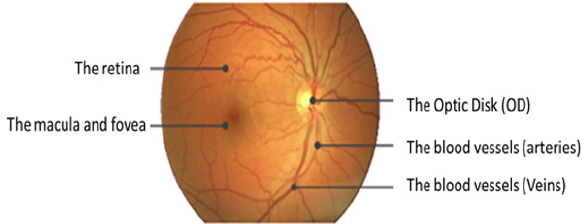
The fundus means back of the lens of the eye. It contains the retina, OD, MA, FV, and posterior pole. Figure 1 shows the anatomy of the normal eye. The retina is the tissue that projects the image. In respect of eye contents, the retina contains light-sensitive cells called rods and cones that are in charge of night and daytime vision, respectively. The OD conveys information of the image comes into the brain. OD is a bright white or yellow circular area in the eye. It is the center point of the vascular tree in a human eye as large blood vessels are found from the OD as shown in the figure. The MA is an elliptical spot on the side of the retina center with a diameter of about 1.5 mm. The FV is close to the MA center. It includes cone cells. The FV is responsible for the accurate vision. It enables us to see the objects and things in more details. On the other hand, the blood vessels consist of the arteries and veins. They have the responsibility of the blood supplement from heart and lungs to the eye and vice versa [4,5].
DR Disease
DR is caused by diabetes and may result in the blindness. It appears in the retina. In this disease, the vessel becomes weak. According to the vessel infiltration, blood and liquid of lipoproteins create abnormalities in the retina. The DR may exist various types of abnormal lesions in a diabetic’s eye. The lesion types are like micro-aneurysm, hard and soft exudates, and hemorrhage. Table 1 shows the description of the DR lesion types. We can notice that some lesions have the same description of some components of the eye; such as the color. For example, the hemorrhages are yellow or white areas or spots in the eye. They are the same as the OD. Moreover, the hard or soft exudates are the same as blood vessels in color. All of that makes the extraction of the lesion from the retinal fundus image is difficult that is considered a challenge to formulate an accurate extraction. In our experimental results and discussion section, we will illustrate our work in the dataset that contains some lesions of the DR, such as hemorrhages, hard and soft exudates, and the small red dots that are like soft exudates but smaller.
The Related Work
This section introduces the findings of the studies in the blood vessels segmentation and ocular diseases classifications. We provide the used framework phases and techniques illustrating the advantages and limitations. Moreover, what they intended to do in the future to develop their work. It is categorized into three subsections. The first one is the supervised methods. The second is the automated method or unsupervised method. The last is the semi-automated methods. On the other hand, we present the fourth section that includes all methods that used both of the structure and color features. Finally, we present the last subsection that includes the results and the discussion about the author’s findings in the four subsections. In the last subsection, we compare the results of the authors who used the same datasets and performance measures.
The Supervised Methods
Diseases differently affect arteries and veins, such as atherosclerosis and hypertension that lead to abnormal blood vessels. They affect the width, length, and diameter of the vessels. For example, cardiovascular (AVR)diseases cause changes in the length of vessels. They increase the curvature or other modification in the vessel’s apparition. Therefore, the separation of arteries and veins is an essential requirement for the classification and diagnosing of most of the ophthalmological diseases. This subsection presents the literature that used the supervised method to segment and classifies the retinal vessels using mainly the structural features of the vessels. Fraz et al. [6] compared between a set of the performance of classification algorithms. These algorithms were applied to two available datasets that are called DRIVE and STARE of retinal images. The comparison was made using the accuracy of classification. From their survey, the authors demonstrated that the supervised methods are better than their counterparts. On the other hand, they do not work well on the noisy images. For the matched filters such as Gaussian matched filters that can be optimized to give better accuracy can be used in automatic blood vessel segmentation helps in the minimizing the runtime. The disadvantages of this survey, most of the techniques presented in the literature were evaluated on small datasets. Most of them included twenty images. The limited range of images not presented for all image characteristics. These characteristics are such as the variability of inter and intra image in luminance, the contrast values and the different values of the gray background level. Fathi and Naghsh-Nilchi et al. [7] motivated their work as the development of automatic blood vessels extraction is very important in diagnosing multiple ophthalmology diseases. The author used the complex continuous wavelet transform (CCWT) as a multi-resolution method to clarify the structures of lines in all directions. Moreover, to separate these lines from simple edges. Besides, the method was used to remove the effect of noise. The authors’ framework was consisted of three phases to extract the blood vessel network. The framework phases were preprocessing, vessel enhancement and vessel detection. The colored retinal image is input to the preprocessing phase. They selected the green channel and inverted it to appear the blood vessels brighter than the non-vessels background. After that, the authors applied the contrast adjustment process on the inverted green channel to enhance image contrast. By using this channel, they could reduce the effect of non-uniform illumination. Besides that, they used the border region expanding algorithm. This technique removed the border of the image to appear only the vessel network. The wavelet method parameters such as frequency and scales were used. Scale 2 was used for thin vessels, and scale four was used for thick vessels. Another technique was used in the vessel enhancement phase was the wave shrink technique to remove noise. Brian et al. [8] introduced a method to differentiate between exudates and hemorrhages diseases in fundus retinal images. They extracted the two diseases to detect the Diabetic Retinopathy DR. They selected the green channel in the pre-processing phase and detected the Optic Disc by using circular Hough transform (CHT). After that, they enhanced the image by using Contrast Limited Adaptive Histogram Equalization (CLAHE). The authors detected the two diseases separately. They combined CLAHE with the Gabor filter and followed by the thresholding to extract the exudates. On the other side, they combined the CHT with the thresholding to detect the hemorrhages. The authors used STARE and DRIVE datasets. In the future, the authors intended to classify different types of DR based. The advantage of the method was that the authors used the Gabor Wavelets that are very beneficial in the retinal analysis. The disadvantages of this method are that the authors segmented the two diseases separately. The image may have the two diseases at the same time. In this case and due to their method, the one image will be entered twice to be detected, one for the exudates and the other for the hemorrhages. Of course, this will waste time and effort and will make conflicts in most cases.
Morales et al. [9] tried to discriminate between the normal and pathology in retinal fundus images. For the pathology, they tried to discriminate between the AMD and DR at the same time without using segmentation. They used LBP as a descriptor for the texture features in retinal images. Their framework started with the preprocessing. In that phase, they resized the images from different data sets to a standard size by using bicubic interpolation. The median filter was used after resizing the images to reduce the noise. They detected the vessels and the OD and excluded them from the LBP neighborhood. The second phase of their framework was the feature extraction. They described retinal background by combining LBP and VAR operators for each component of RGB. They extracted the mean, standard deviation, and other statistic features to be used in classification phase. Before the classification, the authors made data normalization and resembling. They used wrapper method to select the features set. Finally, they made the classification by selecting the classifier to train the selected subset of features. They used four data sets ARIA, STARE, E-OPHTHA, and private data set DIAGNOS. They worked on Weka platform. Their method was evaluated using specificity and sensitivity measures. The experiments were done using different classifiers such as Logistic Regression LR, NN, NB, SVM, C4.5, Rotation and Random Forest and Ada Boost. They used the best classifier gave best specificity and sensitivity results in each experiment. On the other hand, they compared between their method, LBPF and LBQ descriptors. They discovered that using the combination of the three components of R, G, and B information gave the best performance than using only the green channel. The advantage of their work was that they did not use the lesions segmentation before the classification. The disadvantage was that the detection of the DR was so small because this disease is very difficult to be detected through only texture analysis. Moreover, although the wrapper strategy they used was better in feature selection, it was time-consuming than PCA. In the future, the authors intended to test more images in large data sets and would examine more in LBP and other texture descriptors based on co-occurrence.
Nguyen et al. [10] tried to predict the diseases based on the apparition of the vessels. The authors tracked vessels from color retinal images using basic line detector for measuring changing the length the vessels. This reduced the overall accuracy of their proposed method, mostly on STARE images. Their proposed method produced false vessel detection near the OD due to high similarity with pathological regions. They overcome the shortage of the detector by using the line responses. They used the technique at varying scales. They rectified the performance using DRIVE, STARE. In the future, the authors intended to embed the post-processing step to localize dark and bright lesions regions. They wanted to reduce false positives and would apply their method to analyze and detect the vascular tree to detect different diseases. Fraz et al. [6] proposed a supervised method for vessels segmentation in retinal. They used boosted algorithm and utilized a feature vector using Gabor, morphological filter, line strength, and gradient vector. A bagged ensemble classifier was used. They rectified their work on DRIVE and STARE. In classification, they adopted characterization for each pixel. The features used for pixel classification were successfully encoded the retinal information to characterize normal and pathological retinas. They reduced feature space from 9features to only 4, which resulted in less computational time. For future work, vessel width and tortuosity measures are important to be incorporated into the algorithm.
Unsupervised Methods
In automated methods, features are extracted from major vessels. First, the algorithms extract the vascular network from image structures. Then, extract the pixels that are centerlines from the segmented vascular tree. Various features are calculated for each centerline pixel. The classifier can label the two types of vessels. This subsection produces all the automatic techniques that were used in the literature. Azzopardi et al. [1] presented automatic segmentation method for vessel tree as a preprocessing step. It simplifies the processes that contribute to the diagnosis. The authors used B-COSFIRE to detect bar-shaped structures a blood vessel. B-COSFIRE is non-linear as it realized orientation selection by multiplying the outputs of DoG filters. B-COSFIRE is a trainable approach. It means that the selection of the filter is determined from a user. For example, determining a straight vessel, a bifurcation, etc. The author’s used DRIVE, STARE, CHASE_DB1, REVIEW, Bio Im Lab. The authors started the framework by the preprocessing phase to enhance the contrast. Moreover, the preprocessing stage is very important to smooth the edge of the field of view (FOV) of the retina. In this phase, the authors considered only the green channel. They used FOV - mask image to determine the initial ROI in DRIVE database only. But In the other databases, they used thresholding of the CIE Lab version of the RGB. After that, they dilated the border. Finally, they enhanced the image by using CLAHE. The B-COSFIRE procedure consists of detection of changes in intensity, the configuration of B-COSFIRE filter, blurring and shifting DoG responses, achieving rotation invariance and detection of bar endings. The performance measures used in this work were accuracy, sensitivity, specificity, and Matthews correlation coefficient by the experiments, an asymmetric filter realized higher values in the proximity of the bar endings but is less robust to noise than a symmetric B-COSFIRE. The performance comparing to some supervised methods is somewhat less than others. In the future, the proposed filter requires high-dimensional feature vectors for training algorithm to reach the best margin.
Semi-Automated Methods
The ophthalmologists label the premier points of the main vessels. Then using the structural and connectivity characteristics, the labels are proliferating toward smaller vessels. According to structural features of the vascular tree, in a cross over point, an artery, and a vain. That is done because artery or vein never crosses similar vessels. Hatami et al. [11] proposed a Local Binary Pattern-based method (LBP) method for Retinal Arteries and Veins identification in Fundus Images. They utilized LBP to collect the local structure around a pixel by thresholding its neighborhood. They overcame the problems of i.e., rotations of the input image (Rotation Invariant LBP) and small spatial support area, which only considers micro texture information (Multiscale LBP). A Multiple Classifier System was used to handle the complexity of the problem properly. For future work, developing a system that automatically computes AVR diameter ratio. Also, a combination of the proposed method and an automatic algorithm for OD identification. Moreover, classification error rates can be reduced by including meta-knowledge about arteries and vein. Another possible future direction is to combine different features (e.g., ICA) with the LBP features and use it for training the classifier. Including anatomical characteristics of the vessels and vessel position information in the retina could be informative too. The proposed method may not be limited to the retinal vessel it may be possible to apply it to any vascular system. Or it may be applied to any other medical imaging application area.
Lau et al. [12] Used binary trees to find constraints on the vessel trees. The time complexity of graph tracer is exponential to the number of edges. It is not dependent on the retinal image size. It deals only with the connection of entire segments. These segments discarded pixel measuring such as intensity. Moreover, it neglected using pre-processing steps of enhancement or separation of arteries and veins. The thing that is so important for the system. For accurate classification, AVR is estimated from the segmented region of interest of vessels. In addition to the mean diameter of vessels in each class. Itis calculated of final AVR. The automated method which combines color and structural features of vessel networks. In which vessels in the region can be determined based on features such as color, the width of vessels, etc. Since biological characteristics of the personlead to a change in the color of the retina which raises another problem.
Combining Structure and Color Features
In this subsection, we present the techniques available in the literature that depended on the extraction of color and structure features. They combined with these features to achieve maximum accuracy. Mirsharif et al. [13] presented a method that first employed the enhancement by using CLAHE to improve the images. Then they used Gabor wavelets for feature extraction to separate major arteries from veins. They concentrated on the classification of vessels in ROI for AVR. They employed correlative information at crossover and bifurcation. By this information of points, they could revise some vessels that were mislabeled. They evaluated their results on the available DRIVE dataset. On the other hand, they put into an account to decrease the number of the training sample points and features. They classified the vessel segments rather than segmenting the vessel points. They investigated features in RGB, HSL, and LAB. The advantages of their work were that they presented an automated method which combined color and structural features of the vessels tree. The authors Performed clustering in each region independently, comparing to clustering on the whole image. LDA classifier is used. On the other hand, the limitation was that a single classifier is less able to handle the complexity of the problem properly.
Orlando et al. [2] implemented an automatic structured learning method using support vector machine segmenting blood vessel in fundus images. The automatic tools aids in early detection of retinal diseases, while vessels need to be previously detected. Thus, they performed a manual segmentation step aided by trained experts. Their proposed method weighed the pair wise interactions. These interactions were ranked according to the relative distance of each pixel. The authors overcome the problem of scaling images at Different resolution. They computed the unary potentials according to responses to the multi-scale line detectors and responses to 2-D Gabor wavelets features extraction methods. These feature parameters were used to train FC-CRF model. Their proposed learning strategy model exploited the interaction between pixels features than using a local neighborhood-based approach. It resulted in a good performance, with less misclassification. They intended to add development in feature extraction or learning to improve the performance. Fan et al. [14] presented the computeraided framework in order to detect the OD. There is a similarity between OD and the exudates in features such as colour and shape. Therefore, it is very important to detect the OD. On the other hand, detecting the OD affect detection of the glaucoma disease in the part of optic cup size. The author used a supervised method. They ignored the assumptions that can be suggested in the unsupervised methods. They depended on the structure features such as edge information to detect OD of the fundus image.
Their framework consisted of two phases training and testing. It started with training the edge detector such as random forest without selecting any channel of the image. Then, they cropped the image to produce the sub-image with detected points. After that, the authors used the Laplacian of Gaussian as a correlation filter. Therefore, they extracted the features vector. In the structure learning, they predict the structured objects rather than real values. Moreover, they used the ground truth to adjust the model. The output of the first phase was the local segmentation mask and the OD edge map. In the second phase, they cropped the tested images and extracted the features. Then they applied the structured classification. After that, they employed the thresholding to produce the binary image and applied the circle Hough transform on it to detect the OD shape. They applied their framework to three datasets, MESSIDOR, DRIONS, and ONHSD. They used the images in the last two datasets as training dataset and the images of the first one as the testing dataset. When they used the images on the first dataset as training dataset and tested on the last two datasets, they obtained the desired results but not achieve the results when doing the vice versa. The reason for that was, the images in the first dataset were very larger than in the combination of the others, so, the disadvantages here were that MESSIDOR contained different local structures. If they used the images on DRIONS and ONHSD to train the model, many local structures on MESSIDOR could not be captured during training. On the other hand, the trained model is unable to synthesize novel labels. Therefore, they had to use the first suggestion, although they obtained worst results. The author’s proposed method may be outperformed when they used a large number of patches of features about or larger than 106 to train the forest random. In the future, the author intended to combine the advantages of deep learning and the structured learning. They will be used to train the edge detector to improve their results.
The Related Work Results and Discussions
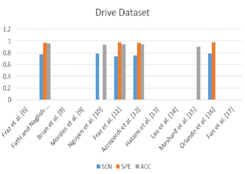
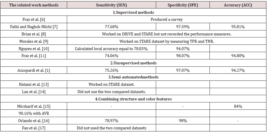
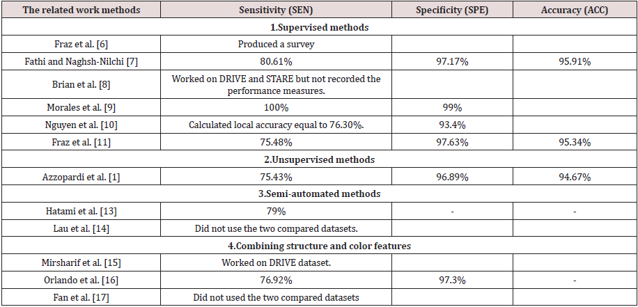
In this subsection, we present the results of the authors in the literature who used the same datasets and the performance measures and provide the discussion and conclusion about their presented results. Tables 2 & 3. Present the results of the related work on the two public datasets DRIVE and STARE using the three performance measures sensitivity, specificity, and accuracy. From Table 2. We can observe that Fathi and Naghsh-Nilchi et al. [7] achieved the best accuracy compared to the others. They achieved 95.81%. This means that the user interaction affects greatly the accuracy but nowadays, we need an accurate automatic method. It is a challenge to achieve accuracy without participating the user. On the other hand, we notice that Fraz et al, [6] as a supervised method also achieved the second-best accuracy compared to the others. Their accuracy was equal to 94.80%, and the specificity was equal to 98.07%. Although Mirsharif et al. [13] combined between the color and the structure features, they achieved accuracy 84% without structure feature and 90.16% with structure feature such as measuring the diameter of vessels by AVR. Their accuracy was less than any of the supervised, unsupervised or semi-automated methods. Figure 2 represents the previous results of the related work methods applied to the DRIVE dataset. The bar chart shows the methods that were proposed and their performance measures due to SEN, SPE and ACC.
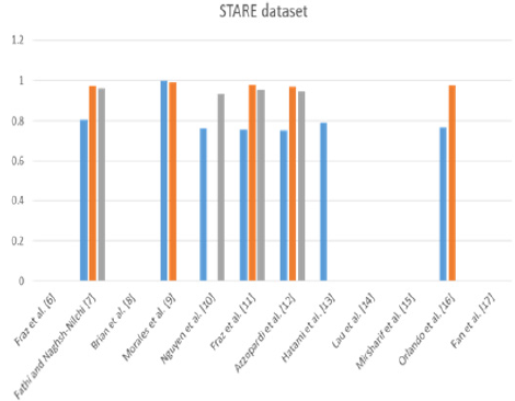
From Table 3. We can observe that Morales et al. [9] achieved best TPR or sensitivity was equal to 100% and the TNR or specificity was equal to 99%. It was also the supervised method. On the other hand, Fathi and Naghsh-Nilchi et al. [7] achieved the second-best accuracy after Morales et al. [9] compared to the others. They achieved 95.91% in STARE dataset. This means that the user interaction affects greatly the accuracy also in the second dataset such as the DRIVE dataset. Again, nowadays, we need an accurate automatic method for diagnosing and detecting the lesions, especially in ophthalmological diseases. On the other hand, we notice that Fraz et al. [6] as a supervised method also achieved the second-best accuracy compared to the others. Their accuracy was equal to 95.34%, and the specificity was equal to 97.63%. Although Orlando et al. [2] combined between the color and the structure features, they achieved sensitivity 76.92% and specificity was equal to 97.3%. Their accuracy was less than any of the supervised, unsupervised or semi-automated methods. Figure 3 represents the previous results of the related work methods applied to the STARE dataset. The bar chart shows the methods that were proposed and their performance measures due to SEN, SPE, and ACC. From the related work, most of the author stake into consideration the structure and intensity feature to detect the vessels and nonvessels. The others used them to detect normal or up-normal. Most of them concentrated on extracting the blood vessels. It is very important but not work in all fundus image dataset such BCOSFIRE, as we will see in section 5. On the other hand, no one of them introduced a method or framework to solve the problem of multilabel classification to detect multiple lesions of diabetic retinopathy simultaneously. In our proposed framework, we present a method to detect multiple lesions simultaneously using algorithm adaptation based on the problem transformation concept. We used MSVM as a multi-level classifier. It detects at first level the normality and upnormality. After that, it outputs the detection of each class. Finally, we combined all the output of the classifiers on all classes of the lesions and calculated the average accuracy.
The Proposed ML-CAD System
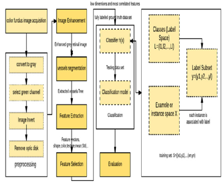
In this section, we illustrate the phases of classifying multiple ophthalmological diseases at the same time using the idea of problem transformation. The proposed multi-label CAD system framework consists of six phases as shown in Figure 4 as following:
Phase 1: Color Fundus Image Acquisition: Fundus images have the advantage that a specialist can examine them at another location or time and provides photo documentation for future reference. The images result from the fundus camera. Currently, available fundus camera scanis categorized into five groups [15].
a) Traditional Oce-Based Fundus Cameras: They have the best image quality, but they are expensive. The operation of such devices is very complex. Therefore, they require highly trained professionals. On the other hand, they require the patient to visit the clinic.
b) Miniature Tabletop Fundus Cameras: They are simple but very expensive and require the patient’s visit to the clinic. Their high cost limits them from a widespread.
c) Point and Shoot Off-The-Shelf Cameras: They are light, hand-held devices. They have low cost and a good image quality. The main limitation of these cameras is the lack of fixation. The reflections from various parts of the eye can hide important parts of the retina.
d) Integrated Adapter-Based Hand-Held Ophthalmic Cameras: They can produce a high resolution, reflection free image. The bottleneck is the manual alignment of the light beam, which makes image acquisition highly time-consuming.
e) Smart-Phone Based Ophthalmic Cameras: They emerge from the continuous development of the mobile phone hardware. The application of such devices may have a major impact on clinical fundus photography in the future. The main limitations of it are rooted in its hand-held nature: focusing and illumination beam positioning can be time-consuming. However, despite that their performance is not yet assessed in comprehensive clinical trials, these devices show promising results.
Phase 2: Pre-Processing: Due to the disadvantages of the most fundus cameras, we should preprocess the images that out from the camera. The images resulting from the fundus camera cannot be analyzed clinically. At least for one eye. The reasons for that are insufficient image quality. The causes of poor image quality are the non-uniform illumination, reduced contrast, media opacity and movements of the eye. Therefore, the images that are resulted from the fundus camera are entered to the preprocessing phase in our proposed framework. The preprocessing phase consists of some steps such as converting the color fundus image to a gray level. When we make the conversion, we can find red, green, and blue channels. We selected the green channel because it is brightest and more contrast than other channels. After that, we made the inversion. The previous step is done if we want to extract the blood vessels in the segmentation phase. Then, we remove the OD from the image. As we mentioned before in section 2, the OD should be eliminated because it has the same features such as intensity as the same ashard exudates lesion. Finally, we enhanced images by CLAHE. The results will be shown in the next section. In CLAHE, the contrast of an image is enhanced by applying CLHE on small data regions rather than the entire image. CLHE is based on thresholding and equalization. Using the inter polation which is bilinear, the resulting neighboring tiles are stitched back seamlessly. The contrast in the homogeneous region can be limited so that noise can be avoided.
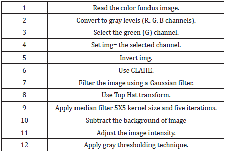
Phase 3: Blood Vessels Segmentation: Extracting the blood vessels is very important in detecting most of the ocular diseases. Because of the up-normality of the blood vessels leads to the type of the lesion. On the other hand, the accuracy of classification depends greatly on the segmentation. In some datasets such as DRIVE and STARE we can use the BCOSFIR [1] to extract the blood vessels. But in the other datasets such as the used dataset in our experiments DIARET db dataset. This method cannot extract the blood vessels completely as we will see in the next section. Therefore, we made some steps as shown in Table 4. As an alternative, we can use Fuzzy-c-means to extract the cluster of the blood vessels. In this phase, we should extract the areas of the hard or soft exudates and hemorrhages. These areas are the focused ROI that we need to extract their features. If the dataset has the ground truth images, therefore, we can use the ground truth in training dataset without segmentation to evaluate the accuracy of the classifier. In general, we need to make accurate segmentation to apply the framework on any collected retinal fundus images that may not have ground truth. To extract the exudates, we used the same steps in Table 4. But with using the morphological structure by using steel (ball) and wavelet transform. The same thing for extracting the hemorrhages.
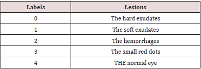
Phase 4: Feature Extraction: We extracted the features of the segmented images in the training steps to introduce the feature vector that will be entered into the classifier. We used the gray level Co-occurrence matrix (GLCM). We used 13 features for the 89 images of the DIARET dataset. The features are Contrast, Correlation, Energy, Homogeneity, Mean, Standard Deviation, Entropy, root mean square (RMS), Variance, Smoothness, Kurtosis, Skewness [16]. The GLCM functions characterize the texture of an image. It calculates how often pairs of the pixel with specific values and in a specified spatial relationship occur in an image. It extracts the statistical measures. We calculated the functions of GLCM on MATLAB 2017b platform and recorded the results for the 13-feature vector in the array to the .mat file by looping on the 89 image of the dataset. The resulting mat file is defined as the training features will be entered into the classifier to match the features with the testing images. In this phase, we also construct the mat file for labels that are four labels according to the four lesions hard exudates, soft exudates, hemorrhages and small red dots.
Phase 5: Feature Selection: We used principal component analysis (PCA) to select the most correlated features in order to reduce the dimensionality. This phase is done before the classification. It analyzes a data table. This table in which the observations are described by several dependent variables that are inter-correlated quantitatively. Its objective is to extract the important information from the table. It does the extraction to represent it as a set of new orthogonal variables. These new variables are called principal components PC. PCA displays the pattern of similarity of the observations and the variables as points in maps [17]. The quality of the PCA model can be evaluated using cross-validation from MATLAB 2017bplatform.
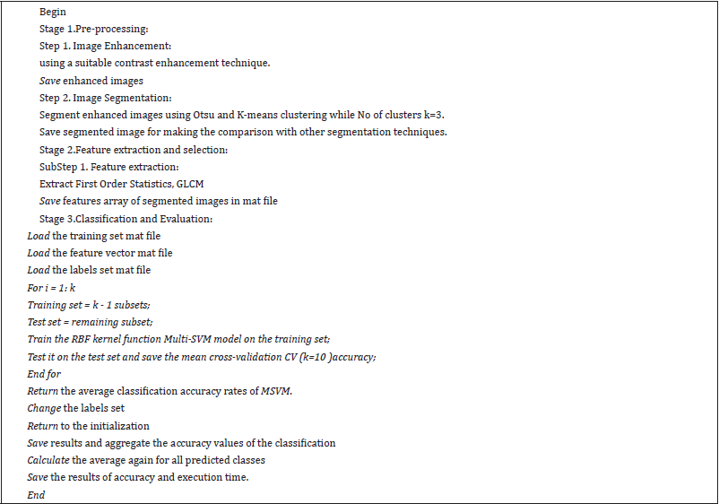
Phase 6: Classification: We used the MSVM. The first level is to determine if the eye is normal or up-normal. The other levels are to determine the type of lesion through the classes of the lesions. Therefore, before demonstrating the classification phase in the proposed multi-label CAD system framework, we provide at first the types of multi-label classification methods then illustrating the technique of MSVM idea.
An Overview of Multi-Label Classification Methods
There are a lot of methods developed for multi-label classification. The current methods are based on two basic approaches. The first approach is algorithm adaptation and the second is problem transformation. Another type of multi-label method is the ensemble methods. They combine outcomes from several classifiers based on either problem transformation or algorithm adaptation. The algorithms are such as RAkEL.
a. Algorithm adaptation: It is the extension of the traditional methods to perform multi-label classification directly. The classifiers that use algorithm adaptation, such as Adaboost.MH in ensembles methods and ML-KNN in instance base methods [18].
b. Problem Transformation: It transfers multi-label classifications into multiple single labels. Then, all the classification algorithms can be applied directly for each binary dataset. The outputs of the binary classifiers are then aggregated for the prediction. The classifiers that use problem transformation are such as BR, CC in binary methods and PS in label combination methods [18]. The methods of this strategy are simple and computationally efficient if put into consideration the label independence. They are expensive in the computation if care about label relationships, such as LP. Methods from this category are algorithm independent.
MSVM
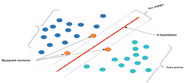
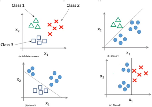
SVM splits the data points into two classes. The separating line or a hyper plane is the best possible way because it gives the widest road or margin to separate the two groups of data into zero or one, or as healthy or not as in our work. The margin is needed between the two classes in order to reach the separation accurately. The distance between the points and the line are as far as possible. Therefore, these points are called support vectors. The SVM problem is to find the decision surface which maximizes the margin in a training set. The support vectors are the effective points in the training process. Figure 5 illustrates the SVM idea. Figure 5 shows the data points that need to be separated or classified using the linear SVM. The hyper plane best separates the data points putting into account the maximization of the margin. The effective elements that will be used are the support vectors while the far points will be excluded. In multiclass SVM, it decomposes the problem into a set of binary problems, in this case, the binary SVM can be directly trained. The two approaches of SVM are one-versus-rest (OVR) and one-versusone (OVO). Both of them decompose the problem into some binary problems. Then, they combine binary-class problems into one single objective function and simultaneously realizes classification of many classes. We used the first scheme. It constructs S binary classifiers for S-class. Each binary classifier is trained using the data from the specified classes as positive instances and the remaining S − 1classes as negative instances. In testing, the binary classifier determines the class label which gives maximum output value. A main problem of OVR is the imbalanced training set. The problem is solved if all classes have similar size of the training instances, then the ratio of positive to a negative instance in each classifier is 1/S−1. Figure 6 illustrates the OVR approach. From Figure 6 The image on the top left shows the three classes of data class (1,2 and 3) that should be separated using MSVM with the approach of OVR. The classifier work with each class against the rest. It considers each class is positive and the rest are negative.
MSVM
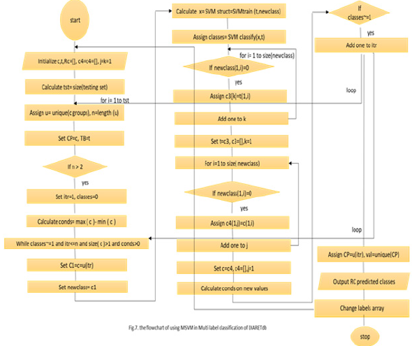
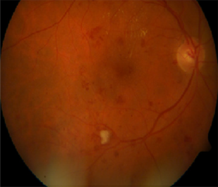
Figure 7 Shows the flowchart of using MLSVM in multi-label classification. At first, we initialize the training set (t), the groups (c and the testing array. It results in the predicted classes. As the processes, the size of the testing set is calculated. The loop is made till the calculated size. In the first loop, we assign the training set and the classes groups putting into account the length of the unique groups to dismiss the similar values in the group. If the unique groups are larger than two then setting the classes equal to zero and subtracting the maximum of groups from the minimum of them. After that and within the outer loop, enter to the nested loop while the condition is achieved. The condition is if the classes are not equal to one and the iteration (itr) is less or equal to the length of unique groups, and the previous subtraction is more than one. Inside this loop, we define new variable c1 which is assigned the value of c and defined also the new class to have the c1 value. We used the kernel RBF function as shown in the flowchart. Then, we open two loops to reduce the training set and the groups. As demonstrated before, the feature vector is entered to the MLSVM classifier with labels and the test images group tables. The classifier makes the iterations and detects the disease in the entered image. Of course, that is done due to the matching of features. It determines the class of the entered retinal image. It determines if the image has hard or soft exudates, or hemorrhages, or small red dots the set of labels. There are some images in DIARET db dataset contain the four lesions as shown in Figures 8 & 9. Figure 8 shows the image in DIARET db dataset which contains the four lesions. Figure 9 Shows the ground truth of the four lesions in the image. Therefore, we executed the classifier in the four classes for all 89 images and combined the results of the classifiers. This method is called problem transformation method of multi-Label classification. In the proposed MLCAD system framework in Figure 4. We demonstrate the multi-label idea. Assume that the label space is ꓡ= {l1,l2,l3,……lL} and the examples or instance space X where x ϵ X. The instance x is relatedto a subset of labels У where У is a part of or equal to the label space. The label set can be represented by a vector Y= (y1,y2,….,yL). If yi=1 that indicates the label li is relevant to for the given instance. If yi=0 then the label li is not relevant to the given an example. Through the training set S= {(x1,y1), (x2,y2),..., (xn,yn)}, the classifier h carries out the mapping h: x→L that were generalized beyond the training set. In classification, when the system is composed of a separate classifier per class such as h(x)=(h1(x), h2(x),….,hL(x)), each binary classifier hi(x) assigns the prediction yiϵ{0,1} to the example x. As a common meaning, the training set consists of the instance whose known class labels is provided. The training set is used to build the model which is posteriorly implemented to the test set. The test set consists of the instances with unknown class labels. The test set is the images that will be detected in such four classes Table 5. Define the pseudo code of the overall classification.
Phase 7: The Evaluation
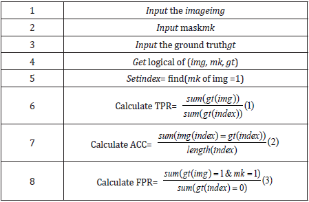
We evaluate our framework using the accuracy, true positive ratio (TPR), and the false positive ratio (FPR) [3,19]. The Accuracy, TPR, and FPR are calculated by equations 1,2, and 3 that are showed in the following pseudo code in Table 6.
Table 6: The Accuracy, TPR, and FPR are calculated by equations 1,2, and 3 that are showed in the following pseudo code table.
The Experimental Results
This section includes the methods and material used in our work. Moreover, we recorded the results of the experiments we did. The results are illustrated in the second subsection. Finally, the last subsection presents the discussions about the experimental results. n this work, we used the multi-label retinal fundus images dataset called DIARET db. It is a standard DR dataset. It consists of 89 color fundus images with the extension of (PNG). Five of them are considered normal that does not contain any sign of DR due to the experts who participated in the evaluation. The rest of images that counts eighty-four contain at least mild non-proliferative signs Micro aneurysms of the DR. The images of the dataset were captured using the same 50-degree field-of-view digital fundus camera with varying imaging settings. The dataset can be used to evaluate the general performance of diagnostic methods. This dataset is referred to as “calibration level 1 fundus images”. On the other hand, the dataset contains the ground truth for all images in the four signs of the DR hard, soft exudates, hemorrhages, and small red dots or Micro aneurysms [3]. On the other hand, we used MATLAB 2017b platform. We used 20 images of the DIARETdb. At first, we should assume that there is no ground truth for the used dataset because we intended to apply our framework to another dataset that will be established or collected from other ophthalmological centers or hospitals. Therefore, we made a segmentation phase in our framework and matched its results with the ground truth. There are some images in the dataset need to be segmented to extract the blood vessels. On the other hand, the other images need to be segmented to extract the areas of the four lesions as we administrated before. To extract the blood vessels, we used the BCOSFIR [1], but it did not work with the used dataset although it works will with DRIVE and STARE datasets [20]. Figure 5 shows the difference between BCOSFIRE and our blood vessel segmentation steps. Figure 5 shows the three images from left to right. The left image is the original color fundus image number (image_022) [21]. The medium is the BCOSFIRE blood vessel extraction, and the left is our blood vessel extraction.
Figure 9: The found truth of the four lesions in the DIARETDB image (a) Hard (b) soft exudates (c) hemorrhages and (d) Microaneurysms.
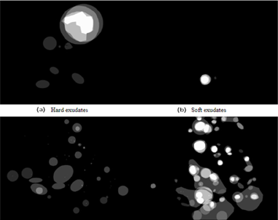
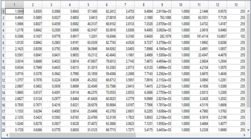
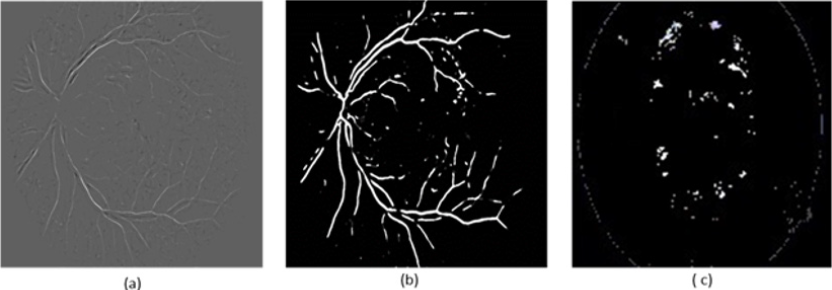
As shown in Figure 10, we observed that our segmentation method extract the blood vessels more accurate than BCOSFIRE. Figure 11 shows the same results but for image number (image_005). As shown in Figure 10, we can observe that BCOSFIRE shows the blood vessels but not all the vascular tree, the thing that can affect the classification accuracy [22]. We started our proposed framework by converting the color fundus image into gray level images with the three channels as shown in Figure 12. We selected the green channel because it is more contrast than other channels. After that, we inverted it to make the blood vessels to be brighter, as shown in Figure 12 & 13 shows using the CLAHE and the Gaussian blur filter respectively. After that, we applied the segmentation steps that was illustrated in Section 4 [23]. On the other hand, when wanted to extract only the lesion that was shown in the ground truth of DIARET db dataset as in Figure 9. We used K-means and Otsu’s Thresholding as shown in Figure 14 for the image_005. After we segmented the ROI areas, we extracted the features using the GLCM. We extracted 13 features as shown in Figure 15. It shows the snapshot of the features vector of 20 images of the DIARET db dataset in MATLAB 2017b. The first row has the numbers of features that are ordered as [Contrast, Correlation, Energy, Homogeneity, Mean, Standard Deviation, Entropy, RMS, Variance, Smoothness, Kurtosis, Skewness]. Besides that, we created a mat file for labels. We recorded towards each image the label of the lesion it contains as shown in Table 7. After we applied the MSVM, we recorded the accuracy and the training time. Then, we changed the labels of images that have more than one lesion. Again, we recorded the accuracy of each run of the classifier. We combined the results and calculated the average accuracy. Moreover, we applied the other classifiers such as K Nearest Neighbors KNN and ensemble boosted tree and linear SVM. We observed that our method MSVM classifier based on the idea of multi-label classification outperforms the other classifiers in accuracy as shown in Table 7.
Figure 10: (a) The original image_022, (b) BCOSFIRE segmentation and (c) our image_022 segmentation.
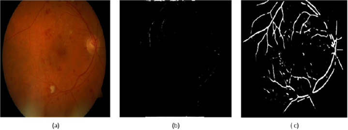
Figure 11: (a) The original image_005, (b) BCOSFIRE segmentation and (c) our image_005 segmentation.
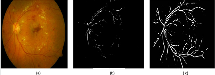
Figure 14: (a) The morphological transform (b) Blood vessels extraction (c) Clustered lesion by kmeans and Otsu’s Thresholding.
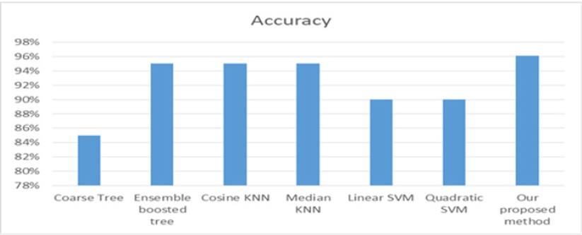
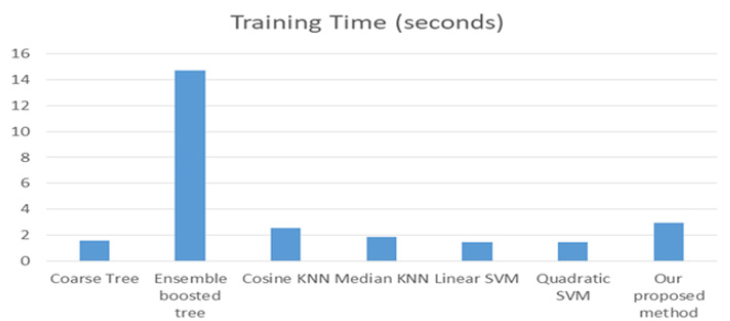
The multi-label classification contributes in appearing the hidden patterns. The correlation among the labels is very important in the ideas of the multi-label classification. From Table 7. We can notice that the accuracy of the proposed method on the DIARET db dataset is 96.1%. The accuracy is greater than the others. The second order of accuracy is KNN, and the ensemble boosted tree. They achieved 95%, but ensemble boosted tree takes a lot of time in training. It takes about 14.7 seconds in comparison to other classifiers. The third level of accuracy is 90% that is achieved by SVM while the average training time is approximately 1.43 seconds. The worst accuracy was achieved by a coarse tree; it was 85%. Figure 16 shows the representing of the accuracy results for all classifiers. It illustrates that the highest accuracy result is of our proposed method followed by KNN and ensemble boosting tree, then SVM and the last level of accuracy is a coarse tree. Figure 17 shows the representation of the training time results of all classifiers applied on DIARET dataset. The longest training time is taken by the ensemble boosted tree. The other training time results are very near to each other. In the range of the other classifiers, our proposed method take longest training time than cosine KNN. The shortest time is taken by linear SVM.
The Discussion
From the previous section, we observed that our proposed method outperformed another state-of-the-art classifier in detecting the multiple eye lesions. Although it achieved the highest accuracy than others, it couldn’t detect the multiple lesion in the image directly. We trained MLSVM for each label. Then we combined the outputs and calculated the average accuracy. On the other hand, we do not trust completely that it combines the correlations between all labels because of the separation of the training of each class.
On the other hand, we should develop an accurate automatic segmentation method to cluster the lesions and the blood vessels. We had to segment the same image twice with two segmentation techniques. Moreover, we should use strong filter to remove noise without effect the details of the image. In this work, we used the Gaussian filter to blur the edges. Besides that, we also used the median filter to remove pepper and salt noise from the segmented image.
Conclusion
The identification of the vessel’s characteristics, such as width, length, diameter, tortuosity, angels, and branches patterns help in diagnosing and defining the ophthalmological diseases, such as diabetic retinopathy or hypertension. Right segmentation of blood vessels leads to accurate classification while the structure and appearance of the arteries and veins determine the disease. In this work, we applied the idea of multi-label classification to detect the multiple diseases in the same fundus image. There are two categories of multi-label classification methods. The first is the direct methods or the algorithm adaptation. The second is the indirect methods or the problem transformation methods. In this chapter, we combined between the two categories to detect the four signs of the diabetic retinopathy disease. They are the hard, soft exudates and the hemorrhages. We used the direct technique in the concept of the problem transformation to achieve the accuracy. The proposed Multi-label CAD system framework starts with the pre-processing, then the segmentation. After the ROI is extracted, we made the feature extraction by using GLCM. After that, we applied PCA to select the features and reduce the dimensionality. In the classification, we applied the MSVM based on the concept of the problem transformation. In the classification phase, we combined the outputs of applying MSVM on each problem and computed the average of accuracy. Finally, we evaluated the proposed method and compared the results due to accuracy and training time with another state-of-the-art classifiers. The proposed method achieved the highest accuracy. We applied the proposed method on the public dataset which is called DIARET db dataset. Our proposed method achieved 96.1% accuracy with mild training time. In the future, we will establish new fundus images dataset with a huge number of images. It will provide different characteristics helping in producing new labels that will lead to high accuracy and avoiding any misclassification. On the other hand, we will develop a classifier that directly detects the multiple ocular diseases simultaneously putting into account the correlations between labels. Also, we will develop an accurate segmentation technique for color fundus images.
References
- Azzopardi G, Strisciuglio N, Vento M, Petkov N (2015) Trainable COSFIRE filters for vessel elineation with application to retinal images. Medical Image Analysis 19(1): 46-57.
- Orlando JI, Prokofyeva E, Blaschko MB (2017) A Discriminatively Trained Fully Connected Conditional Random Field Model for Blood Vessel Segmentation in Fundus Images. IEEE Transactions on Biomedical Engineering 64(1): 16-27.
- Aldrees A, Chikh A (2016) Comparative evaluation of four multi-label classification algorithms in classifying learning objects. Comput Appl Eng Educ 24(4): 651-660.
- Allam A, Youssif A, Ghalwash A (2015) Automatic Segmentation of Optic Disc in Eye Fundus Images: A Survey. Electronic Letters on Computer Vision and Image Analysis 14(1): 1-20.
- KKM, SKN (2013) Review on Fundus Image Acquisition Techniques with Data base Reference to Retinal Abnormalities in Diabetic Retinopathy. International Journal of Computer Applications 68(8): 0975- 8887.
- Fraz MM, Paolo R, Andreas H, Bunyarit U, Alicja RR, et al. (2012) An ensemble Classification-based approach applied to retinal blood vessel segmentation. Trans. Biomed 59(9): 2538-2548.
- Fathi A, Naghsh Nilchi AR (2013) Automatic wavelet-based retinal blood vessels segmentation and vessel diameter estimation. Biomedical Signal Processing and Control 8(1): 71-80.
- Biran A, Sobhe B, Raahemifar K (2016) Automatic Method for Exudates and Hemorrhages Detection from Fundus Retinal Images. WASET. Int J Comp 10(9): 1571-1574.
- Morales S, Engan K, Naranjo V, Colomer A (2017) Retinal Disease Screening Through Local Binary Patterns. Journal of Biomedical and Health Informatics 21(1): 184-192.
- Nguyen UTV, Bhuiyan A, Park LAF, Ramamohanarao K (2013) An effective retinal blood vessel segmentation method using multi-scale line detection. Pattern Recognition 46(3): 703-715.
- Hatamia N, Goldbaum MH (2015) Automatic Identification of Retinal Arteries and Veins in Fundus Images using Local Binary Patterns. Elsevier 1-23.
- Lau QP, Lee ML, Hsu W, Wong TY (2013) Simultaneously Identifying All True Vessels from Segmented Retinal Images. IEEE Transactions on Biomedical Engineering 60(7): 1851-1858.
- Mirsharif Q, Farshad T, Hamidreza P (2013) Automated characterization of blood vessels as arteries and veins in retinal images. Comput Med Imaging Graph 37(7): 607-617.
- Fan Z, Rong Y, Cai X, Lu J, Li W, et al. (2018) Optic Disk Detection in Fundus Image Based on Structured Learning. IEEE Journal of Biomedical and Health Informatics 22(1): 224-234.
- Besenczi R, Tóth J, Hajdu A (2016) A review on automatic analysis techniques for color fundus photographs. Computational and Structural Biotechnology Journal 14: 371-384.
- Gadkari D (2004) Image Quality Analysis Using Glcm.
- Wold S, Kim E, Paul G (1987) Principal component analysis. Chem Intel Labor Sys 2: 37-52.
- Tawiah CA, Sheng VS (2013) Empirical Comparison of Multi-Label Classification Algorithms. Proceedings of the Twenty-Seventh AAAI Conference on Artificial Intelligence 1645-1646.
- Fraz MM, Remagnino P, Hoppe A, Uyyanonvara B, Rudnicka AR, et al. (2012) Blood vessel segmentation methodologies in retinal images - A survey. Comput Methods Prog Biomed 108(1): 407-433.
- Kauppi T, Kalesnykiene V, Kamarainen JK, Lensu L, Sorri I, et al. (2007) The DIARETDB1 Diabetic Retinopathy Database and Evaluation Protocol.
- https://www.drugs.com/cg/retinal-hemorrhage.html
- https://www.isi.uu.nl/Research/Databases/DRIVE/
- Abdel Maksoud E, Elmogy M, Al Awadi R (2015) Brain tumor segmentation based on a hybrid clustering technique. Egyptian Informatics Journal 16(1): 71-81.


