


Lupine Publishers Group
Lupine Publishers
ISSN: 2641-6921
Research Article(ISSN: 2641-6921) 
The Pressure-Temperature Phase Diagram Assessment for Magnesium Hydride Formation/Decomposition Based on DFT and CALPHAD Calculations Volume 4 - Issue 1
Received: April 2, 2021; Published: April 20, 2021
*Corresponding author: Viorel Chihaia, Institute of Physical Chemistry, Ilie Murgulescu, Romanian Academy, Splaiul Independentei 202, Bucharest, Romania
DOI: 10.32474/MAMS.2021.04.000180
Abstract
In this work, we investigate the formation/decomposition boundaries in the P–T phase diagram of the magnesium hydrides. The formation/decomposition boundaries are obtained based on the Gibbs free energy determined by DFT and CALPHAD calculations for the most stable polymorphs of magnesium hydride (α-H2, γ-H2, and ε-H2), of the hcp polymorph of the crystalline magnesium, and of the hydrogen gas (in the real gas model) in the pressure and temperature ranges 0-10 GPa and 0-1200 K, respectively.
Keywords:Magnesium Hydride; magnesium; hydrogen molecule; density functional theory; thermodynamic calculations; P-T phase diagram; formation/decomposition boundaries
Introduction
One of the most promising classes of materials for the mobile storage of hydrogen is the chemical compounds of hydrogen with metals, so-called metal hydrides [1]. In particular, the magnesium hydride is a cheap material, with a high theoretical hydrogen weight content (7.6 wt.%) and good reversibility [2]. However, the poor kinetic and thermodynamic properties of magnesium require high ab- and de-sorption temperatures. Reducing the size of the magnesium grains to the nanoscale [3,4], confining [5], alloying [6] and mixing with additives [7] and catalysts [8] are practical solutions for improving the reaction speed at lower temperatures. Very often these solutions are combined [4,9]. The knowledge of the dependence of the magnesium-based hydride stability and phase transitions on the pressure and temperature is important to find the proper paths for the formation and decomposition of magnesium hydride phases and be helpful to guide the experimental investigations [10]. The electronic structure calculation methods based on several approximations of the Schrödinger equation reached nowadays a high level of maturity, being able to calculate the total energy and its derivatives, the structural, mechanical, electric, magnetic and spectral properties for molecular and periodic systems, by quantum chemistry and solid-state methods, respectively. The density functional theory (DFT) is an electronic structure method that considers the electron correlation at a low computational cost and provides accurate results [11]. The highquality calculations of the vibration frequencies for non- and periodic systems in various approximations (harmonic [12], quasi harmonic [13], and anharmonic [14]) permit the calculation of the thermodynamic properties (enthalpy, entropy, and Gibbs free energy) for different composition, pressure (P), and temperature (T) conditions, which can be used to predict the system phase diagram [15].
The total energy-based thermodynamic calculations were essential in predicting and guiding the experimental investigations for determination of the phase diagrams for magnesium [15,16] and hydrogen [17], and it can be applied with success to the magnesium hydride. The CALPHAD (Calculation of Phase Diagrams) calculations of the pressure - hydrogen content [18,19] and temperature - pressure [19] phase diagrams for the magnesium hydride reproduce the experimental data at low pressure (below few tens of MPa). Except for a few studies that consider the real gas model [20,21] most of the thermodynamic theoretical works consider the ideal gas model for the P-T hydride phase diagram [19,22-25]. As far we know there are no experimental or theoretical phase diagrams for the formation/decomposition of the magnesium hydrides at high pressure. In a previous study (Ref. [26]) we performed DFT-based thermodynamic calculations to build the P-T phase diagram of six magnesium hydride polymorphs α-H2, β-H2, c-H2, γ-H2, δ’-H2 and ε-H2 in the pressure and temperature ranges of 0-10 GPa and 0-1200 K, respectively. Here we present the complete P-T phase diagram of the magnesium hydride by calculation of the Gibbs energy for the crystalline hcp-magnesium and the real gas model for the molecular hydrogen and the identification of the formation/decomposition boundary of the magnesium hydrides for the same pressure and temperature ranges as in the previous study. (Ref. [26].
Computational Methods
The thermodynamic properties for the most stable magnesium hydride polymorphs α-H2, γ-H2 and ε-H2 are taken from the previous study [26], which were determined by a high accuracy DFT calculation scheme (plane-wave ultrasoft pseudopotential, exchange-correlation functional PBE [27], energy cutoff of 55 Ry, Brillouin zone - discretized by Monkhorst-Pack scheme [28], with a spacing of 0.04 Å-1). The quality of the used calculation scheme is validated by the confirmation of the coexisting curve of α and γ polymorphs of H2 by DFT thermodynamic calculations [24] and experimental data [29,30]. Recently, the hypothetical cubic structure c-H2, which was found in our calculation to have higher Gibb’s energy than the other considered magnesium hydride polymorphs, was identified by experimental investigations [31] to be metastable as nanocrystal as we supposed in Ref [26]. The used DFT calculations scheme for the three metallic polymorphs hpc, bcc, and fcc of the magnesium is similar as the one used for the magnesium hydride polymorphs, but with a higher energy cutoff (60 Ry) and denser discretization of the Brillouin zone (with a spacing of 0.01 Å-1). The optimized crystalline structures are presented in the Supplementary Information. The phonon and thermodynamic calculations for the magnesium polymorphs are done following the same quasi-harmonic procedure [32] as in the previous article [26]. The Gibbs free energies for the different values of the pressure and temperature were calculated by the Phase GO toolkit, [33] using the data (volume, energy, and the phonon density of states) provided by the thermo_pw calculations with Quantum Espresso [34]. In the case of the crystalline systems, the product pressure-volume in the Gibbs is very small compared with other contributions to the Gibbs energy. However, we considered its contribution to the Gibbs energy.
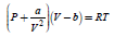
Despite the inability of the DFT method to predict accurately the band gaps, the electron correlation effects at long-range distances and the electron transfer at very high pressures, it gives good results for low pressures of the hydrogen molecules in fluid and crystalline systems even neglecting the nuclear quantum effects, especially using the PBE exchange-correlation potential [35]. The electronic structure and the vibration frequency of the hydrogen molecule were calculated by the Quantum Espresso code through the interface ase.calculators.espresso of the ASE package, using the same calculation scheme as for crystalline H2 and Mg, but reducing the reciprocal space to only the Γ point . To reduce the energy interaction between the hydrogen molecule and its periodic images, the H2 molecule was introduced into a large 20×20×20 Å3 cell. The interatomic distance, dissociation and vibration frequency determined by the chosen calculation schemes are like the experimental and other calculated data. (see in Supplementary Information). The translation and rotation contributions to the Gibbs free energy G(P,T) for the molecular hydrogen gas were calculated for several pressures P and temperatures T using the stereochemistry module of ASE package [36], within the ideal gas model [37]. The pressure corrections [20] to the Gibbs energy of the molecular hydrogen gas coupled with the CALPHAD-type thermodynamic calculations permitted the treatment of the hydrogen as a real gas. The pressuretemperature P-T phase diagram for the formation/decomposition of the magnesium hydride can be built by computing the Gibbs free energy for magnesium hydride, metallic magnesium and hydrogen molecule involved in the reaction,
on various pressure P and temperature T sets. The reaction is at thermodynamic equilibrium and the reactant(s) coexist with the product(s) when the Gibbs free energy of the reactant(s) is equal with that of the product(s). The Gibbs free energy of the crystalline magnesium and molecular hydrogen gas is given by the sum of the individual Gibbs free energies. The metallic magnesium and the hydrogen gas are considered completely separated and the interaction of hydrogen molecules with the magnesium surface is neglected. The thermodynamic properties of the crystalline magnesium are determined by the energy and its derivatives evaluation by solid-state DFT calculations [15,38]. The anharmonic effects are not considered in the present thermodynamic calculations as they become significant above 800 K for the magnesium hydride [23], which is higher than its decomposition temperature. The electronic component of the Gibbs energy is significant only at high temperatures for metallic systems and is neglected in the present study.
Results
For computational reasons, we limit our study to the scenario of the magnesium hydride decomposition into crystalline magnesium and molecular hydrogen gas. The liquid state is not of interest in our case as the magnesium hydride is decomposing by sublimation and not by melting. Moreover, the preliminary calculations at low pressure P = 0.03 Pa indicate the formation/decomposition temperature to be 591.1 K, below 923 K the melting temperature of the hcp magnesium [30]. Despite its simplicity (the lightest element, with one electron and one proton), the hydrogen has a complex P-T phase diagram, which is under continuous updating and debate as more accurate electronic structure methods and more advanced high pressure and temperature experimental techniques become available. A short discussion of the hydrogen phase diagram is given in Supplementary Information.
The Metallic Magnesium
The hcp structure of the magnesium is the most stable one (total energy of -1596.084 eV/atom, followed in stability by the bcc (-1596.080 eV/atom) and fcc (-1596.065 eV/atom) structures as it was predicted by calculations [39] and confirmed by the X-ray diffraction experiments [39,40]. Despite the small difference between the total energies of the three magnesium polymorphs, for the temperature range considered here, the hcp transforms to bcc only at high pressure (above 30 GPa) [16,40-42] and the DFT calculations predict a bcc - fcc transition at a much higher pressure 1260 GPa [42]. As we work at lower pressures P < 10 GPa, only the hcp polymorph of the crystalline magnesium was considered.
.The Gibbs Energy for Hydrogen as a Real Gas
The ideal gas model provides all the ingredients for the calculation of the Gibbs energy together with the electronic structure calculations for a given set pressure-temperature: internal energy, zero-point energy, vibration, translation and rotation contributions to the enthalpy and entropy, which determine the Helmholtz F(P,T) and Gibb’s energies G(P,T): [43,44]

The ideal gas law V=RT/P for the one mole of molecular hydrogen is valid only at pressures around and below standard pressure (Po = 1 bar) and at high temperatures; therefore, it constitutes a limiting case. As the pressure increases the intermolecular distances increases and intermolecular interaction becomes important. At very high pressure, and especially at low temperatures, the gas might condensate into liquid films on surfaces or form drops in the atmosphere. Thus, the development of other P-V-T equation of states not only for gases but also for related liquids and solids is required. In the frame of the real gas model, some corrections must be applied to the ideal gas to include the interactions among the constituents of the gas. Hemmes et al. [45] succeeded to develop an equation of state for the molecular hydrogen based on an extension of the Van der Waals model of the real gas that reproduces the experimental data for the molecular hydrogen for temperatures between 100 and 1000 K and pressures up to 10 Pa.
Starting from the relation

by integration with pressure between the limits Po and P it can be obtained
where Go (T)= G(Po,T) is the Gibbs energy along a reference isobar Po, which usually is considered to be the standard pressure of Po= 1 bar or 105 Pa. The values of the constant pressure heat capacity, enthalpy, and entropy for the pure elements at a lower pressure than the Po are calculated based on the ideal gas model for gases or determined from the experimental measurements for the condensed species and collected in different thermodynamic databases [46]. The molar heat capacities below the standard pressure have a polynomial dependence on the temperature, with good fitting coefficients for different temperature intervals [47], and the Gibbs energy can be evaluated in the CALPHAD calculations using the empiric Shomate equation [48]

The coefficients A-F are determined by the simultaneous fit of the data from the thermodynamic databases and are tabulated in several databases [49,50], which are included in various thermodynamic software. The standard Gibbs energies are referenced to HSER - the enthalpies of the pure elements in their most stable phase (SER – Stable Element Reference) at 298.15 K and 1 bar. The values of coefficients A-F for the molecular hydrogen are given in the Supplementary Information. The dependence of the volume on the pressure given by the Hemmes’s equation of state [45] might be explored to obtain the G(P, T), but this route is difficult to be explored as it gives a 3rd power dependence of volume on pressure. A correction to the ideal gas volume can be introduced because of the gas compressibility as V (P,T ) = RT / P + DV (P,T ) . The experimental data used by Hemmes shows that non-ideal term for molecular hydrogen gas V very small at low pressures and that it is the only pressure dependence. Using this fact, Joubert [20] proposed the correction of the volume with the pressure P described by
where ai, bi and c are constants that can be fitted to the experimental data. Thus, using Eq. 4, the Gibbs energy can be supplied as

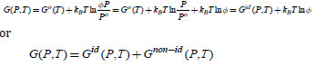
Thus, the Gibbs energy for the real gas can be written as

where
is the Gibbs energy of the ideal gas model, and the residual or excess term?
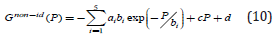
describes the non-ideality of the gas. The values of the coefficients ai, bi, c and d coefficients for molecular hydrogen are provided in, as they are given in Ref [20]. Joubert estimated the constant d G(Po = 1bar,T = 298.15K) = Ho SER in such a way that . A short discussion about the CALPHAD derived Eqs. 3-10 is given in the Supplementary Information. The CALPHAD calculations with Eq. 5 reproduce very well the experimental data of the Gibbs free energy determined for the molecular hydrogen at lower values of the pressure than Po and temperatures above 273.15 K. Thus, together with the correction Gnon−id (P) proposed by Joubert, the experimental and theoretical data for higher pressure given by Hemmes et al. [45] are reproduced.
The third low is fixing the value of the entropy S(P, T=0 K)=0. Thus, the S(P, T= 298.15 K) can be determined by integration. The DFT calculations correspond to T = 0 K and the Gibbs free energy G(0 K)=H(0 K)=Uo+PV is dependent on the calculation scheme through the total energy Uo. Therefore, the reference of HSER has to be shifted by HSER-HDFT to use Eq. 5. Thus, the shifted Eq. 5 for Po is superposing over Go(T) calculated by DFT. We prefer to use it to describe the Gid (P £ Po,T) and the pressure dependence Gnonid (P) given by Eq. 10. The components of the Gibbs energy (total energy, the vibration contributions to the Helmholtz energy, and the translation and rotation contributions to the enthalpy and entropy) for the ideal gas were calculated by the Quantum Espresso program through the module ase. calculators. espresso of ASE package, and the pressure-dependent non-ideal corrections are added by the Gnon-id (P) as described by the Eq. 9 (Figure 1). The component Gnon-id(P)
becomes negligible for pressures P ≤ Po and the hydrogen gas behaves as an ideal gas.Figure 1: The three-dimensional representation of the Gibbs energy G (P,T) of molecular hydrogen gas calculated by ideal (blue surface) and real (red surface) gas model.

Magnesium Hydrides Formation/Decomposition Boundary
The energy vs. volume and the phonon-DOS from the Quantum- Espresso calculations for the hcp magnesium and the three polymorphs α-H2, γ-H2 and ε-H2 are manipulated by the toolkit Phase GO [33], which calculates the Gibbs free energies as a function of pressure and temperatures. The Gibbs free energy for the molecular hydrogen is calculated by ASE coupled to the Quantum Espresso in the frame of the ideal gas model and corrected by Gnon-Id (P, T) given by Eq. 10. Because of the numerical problems of the ASE script, for pressure lower than the Po = 10-4 GPa = 1 bar the ideal gas Gibbs energy is estimated by the Shomate Eq. 5. The full phase diagram (Figure 2) is obtained by using the crossing curves (the thin lines) of the Gibbs energy surfaces G (P, T) corresponding to each pair of magnesium hydride polymorph and the sum of the hcp magnesium and molecular hydrogen real gas. Our study predicts that at high pressures the decomposition temperature grows with pressure and cross the α-γ and γ-ε transformation curves of the magnesium hydride at (2.6 GPa, 684 K) and (5.01 GPa, 750 K), respectively. For the entire range of the considered pressure values in the present study, the decomposition curve is below the melting temperature of the magnesium. Therefore, we suppose that the sublimation and not the melting is the key process in the decomposition of the magnesium hydride. At very low pressure of 10-7 GPa, the decomposition of the magnesium hydride starts at a temperature of 509.1 K, which is 10 K lower than that determined by experimental measurements. The decomposition temperature grows fast with the pressure but much slower than as the experimental behavior, with a shoulder at 10-4 GPa and 519.1 K. At P = 0.03 GPa, the maximum pressure investigated by experiment and used for the CALPHAD calculations, the predicted decomposition temperature is 591.1 K, with 252 K lower than the experimental value.
We are aware that despite that we consider the significant corrections of the real gas of the molecular hydrogen; the built P-T phase diagram is not considering some important effects that are present in the real world like the kinetic factors and neglect some phenomena present at the interface hydrogen gas – magnesium-based solid that might displace the formation/ decomposition boundary to higher temperatures. Therefore, we expect some discrepancies in the predicted decomposition curve by the DFT thermodynamic calculations and the experimental data. The formation/decomposition of the magnesium hydride is accompanied by the structural transformations of the magnesium lattice between hcp-Mg and α-H2 during the hydrogen uptake/release, which involves local strains and energy barriers modification that control the kinetics of these processes. The kinetics of the transformation processes are not considered here. The magnesium and magnesium hydride are polycrystalline materials with many local and extended defects, rather than monocrystalline ones as we considered in the present study. The size and nature of crystallites and their grain boundaries are important factors in the formation/decomposition of the magnesium hydride. A hysteresis effect is experimentally observed in the hydrogen absorption and desorption isotherms. The most accepted justification for this effect is the plastic deformation of the material during the formation of hydride, which is missing during the hydride decomposition. Such an effect is not considered in our calculations.
Figure 2: The formation/decomposition P-T phase diagram of the magnesium hydride. The curves represent the crossing of the Gibbs energy surfaces projected into the P-T plane: α-γ - blue line, γ-ε- green line and formation/decomposition -red line. The dotted blue line with empty dots indicates the DFT calculated α-γ separation line [24] and the blue rhomb and yellow circle indicate two experimental α-γ separation points. [29,30] The inset presents the low-pressure formation/decomposition lines, where the green line with dots indicates the experimental and CALPHAD calculated data for the magnesium hydride decomposition [19] and the red line the calculated data in the present study.

The defects formation and accumulation by ball milling facilitate the diffusion of the hydrogen atoms through the magnesium lattice and the transformation of the lattice, lowering the energy barriers for the formation/decomposition of the magnesium hydrides. The surface morphology and the presence of the passivation films of MgO and Mg(OH)2 when the materials are exposed to the atmosphere delay the penetration or release through such films. When the magnesium is exposed to the environmental atmosphere the passivation layers of magnesium oxide and hydroxide thin films are formed on the top of magnesium and magnesium hydride affect the kinetics of the magnesium hydride formation and decomposition, respectively, shifting these processes to higher temperatures than the temperatures determined by thermodynamic considerations. Despite the important neglected effects, the assessed P-T formation/ decomposition phase diagram for the magnesium hydride can be used to guide the experimentalists to determine a more realistic one and to find a synthetizing way to control the formation/ decomposition phase diagram of the magnesium hydride.
Conclusion
We have performed high accurate thermodynamic DFT calculations by using the PBE exchange-correlation functional for three polymorphs of the magnesium hydride (α−, γ− and ε−H2), hcp magnesium and molecular hydrogen real gas. The Gibbs free energies are computed for different temperatures and pressures and the phase diagram was built from the crossing of the Gibbs energy surfaces of the magnesium hydrides polymorphs and of the hcp magnesium and molecular hydrogen real gas for pressures and temperatures in the range of 0-10 GPa and 0 - 1200 K, respectively. The formation/decomposition curve is starting from 591.1 K for the low-pressure P = 0.03 GPa, growing with the applied pressure in agreement with the findings of the low-pressure experimental investigations and CALPHAD thermodynamic calculations.
Acknowledgment
The work was supported by a grant of the Romanian Ministry of Education and Research, CCCDI - UEFISCDI, project number PNIII- P2-2.1-PED-2019-4816 , within PNCDI III. The authors highly appreciate the support of the Nanotechnology and Advanced Materials research program at EBRC/KISR and the efforts in supporting the research work of computational simulation and modeling for materials science of the Kuwait Foundation for the Advancement of Science. The authors gratefully acknowledge the computing time granted by the Institute of Physical Chemistry “Ilie Murgulescu” on the HPC-ICF infrastructure developed within the Capacities Project 84 CpI/13.09.2007 - National Authority for Scientific Research, Bucharest, Romania. The last two authors acknowledge the financial support for mutual visits provided based on the inter-academic exchange agreement between the Bulgarian Academy of Science and the Romanian Academy.
Additional Information
Supplementary information is available in the online version of the paper.
References
- Demirocak DE (2017) Nanostructured Materials for Next-Generation Energy Storage and Conversion, Eds.: Chen YP, Bashir S & Liu JL pp. 117.
- Jain IP, Lal C, Jain A (2010) Hydrogen storage in Mg: A most promising material. Int J Hydrogen En 35: 5133.
- Pasquini L (2018) The Effects of Nanostructure on the Hydrogen Sorption Properties of Magnesium-Based Metallic Compounds: A Review Crystals 8: 106.
- Zhang J, Yan S. Qu H (2018) Recent progress in magnesium hydride modified through catalysis and nanoconfinement. Int J Hydrogen En 43(3): 1545.
- Konarova M, Tanksale A, Beltramini JN, Lua GQ (2013) Effects of nano-confinement on the hydrogen desorption properties of MgH2. Nano Energy 2(1): 98.
- Cui N, He P, Luo JL (1999) Magnesium-based hydrogen storage materials modified by mechanical alloying. Acta Mater 47(14): 3737.
- Wang Y, Wang Y (2017) Recent advances in additive-enhanced magnesium hydride for hydrogen storage. Prog Nat Sci Mater Int 27(1): 41.
- Webb CJ (2015) A review of catalyst-enhanced magnesium hydride as a hydrogen storage material. J Phys Chem Solids 84: 96.
- El-Eskandarany MS (2019) Recent developments in the fabrication, characterization and implementation of MgH2-based solid-hydrogen materials in the Kuwait Institute for Scientific Research. RSC Adv 9: 9907.
- Kim KC, Kulkarni AD, Johnson JK, Sholl DS (2011) Large-scale screening of metal hydrides for hydrogen storage from first-principles calculations based on equilibrium reaction thermodynamics. Phys Chem Chem Phys 13: 218.
- Wu X, Klein ML, Perdew JP (2016) Accurate first-principles structures and energies of diversely bonded systems from an efficient density functional. Nature Chem 8: 831.
- Alfè D (2009) PHON: A program to calculate phonons using the small displacement method. Comput Phys Commun 180(12): 2622.
- Huang LF, Lu XZ, Tennessen E, Rondinelli JM (2016) An efficient ab-initio quasiharmonic approach for the thermodynamics of solids. Comput.Mat Sci 120: 84-93.
- Hellman O, Abrikosov IA, Simak SI (2011) Lattice dynamics of anharmonic solids from first principles. Phys Rev B 84:180301.
- Li P, Gao G, Wang Y, Ma Y (2010) Crystal Structures and Exotic Behavior of Magnesium under Pressure. J Phys Chem C 114: 21745.
- Althoff JD, Allen PB, Wentzcovich RM, Moriarty JA (1993) Phase diagram and thermodynamic properties of solid magnesium in the quasiharmonic approximation. Phys Rev B 48: 13253.
- Utyuzh AN, Mikheyenkov AV (2017) Hydrogen and its compounds under extreme pressure. Phys Usp 60: 886.
- Bogdanovic B, Bohmhammel K, Christ B, Reiser A, Schlichtea K, et al. (1999) Thermodynamic investigation of the magnesium–hydrogen system. J Alloys Comp 282(1-2): 84-92.
- Zeng K, Klassen T, Oelerich W, Bormann R (1999) Critical assessment and thermodynamic modeling of the Mg–H system. Int J Hydrogen En 24(10): 989-1004.
- Joubert JMA (2010) Calphad-type equation of state for hydrogen gas and its application to the assessment of Rh–H system. Int J Hydrogen En 35(5): 2104-2111.
- Joubert JM (2015) Thermodynamic modelling of metal–hydrogen systems using the Calphad method. J Alloy Compd 645(1): S379-S383.
- Sugimoto H, Fukai Y (1992) Solubility of hydrogen in metals under high hydrogen pressures: Thermodynamical calculations. Acta Metal Mater 40(9): 2327-2336.
- Moser D, Baldissin G, Bull DJ, Riley DJ, Morrison I, et al. (2011) The pressure–temperature phase diagram of MgH2 and isotopic substitution. J Phys Condens Matter 23(30): 305403.
- Yartys VA (2019) Magnesium based materials for hydrogen-based energy storage: Past, present and future. Int J Hydrogen En 44(15): 7809-7859.
- Dornheim M (2011) Thermodynamics of Metal Hydrides: Tailoring Reaction Enthalpies of Hydrogen Storage Materials, in Thermodynamics - Interaction Studies - Solids, Liquids, Gases, Edn Moreno, JC pp. 891.
- AlMatrouk HS, Chihaia V, Alexiev V (2018) Density functional study of the thermodynamic properties and phase diagram of the magnesium hydride. Calphad 60: 7-15.
- Perdew JP, Burke K, Ernzerhof M (1996) Generalized Gradient Approximation Made Simple. Phys Rev Lett 77: 3865.
- Monkhorst HJ, Pack JD (1976) Special points for Brillouin-zone integrations. Phys Rev B 13: 5188.
- Bastide JP, Bonnetot B, Letoffe JM, Claudy P (1980) Polymorphisme de l'hydrure de magnesium sous haute pression. Mater Res Bull 15(12): 1779-1786.
- Toulemonde P, Goujon C, Laversenne L, Bordet P, Bruyère R, et al. (2014) High pressure and high temperature in situ X-ray diffraction studies in the Paris-Edinburgh cell using a laboratory X-ray source. High Press Res 34: 167.
- El-Eskandarany MS, Banyan M, Al-Ajmia F (2018) Discovering a new MgH2 metastable phase. RSC Adv 8: 32003.
- Wang R, Kanzaki M (2015) QHA is able to achieve good accuracy up to the temperature as high as 2/3 of the melting point. Phys Chem Minerals 42: 15.
- Liu ZL (2015) Phasego: A toolkit for automatic calculation and plot of phase diagram. Comput Phys Communic 191: 150.
- Giannozzi P (2009) Quantum Espresso: a modular and open-source software project for quantum simulations of materials. J Phys Condens Matter 21: 395502.
- Morales MA, McMahon JM, Pierleoni C, Ceperley DM (2013) Nuclear Quantum Effects and Nonlocal Exchange-Correlation Functionals Applied to Liquid Hydrogen at High Pressure. Phys Rev Lett 110: 065702.
- https://wiki.fysik.dtu.dk/ase/ase/thermochemistry/thermochemistry.html
- Cramer Ch J (2004) Essentials of Computational Chemistry. Theories and Models. 2nd Edn, (John Wiley & Sons Ltd: 2004): pp. 358.
- Dove MT (1993) Introduction to lattice dynamics Cambridge University Press, USA.
- McMahan AK, Moriarty JA (1983) Structural phase stability in third-period simple metals. Phys Rev B 27: 3235.
- Olijnyk H, Holzapfel WB (1985) High-pressure structural phase transition in Mg. Phys Rev B 31: 4682.
- Mehta S, Price GD, Alfè D (2006) Ab initio thermodynamics and phase diagram of solid magnesium: a comparison of the LDA and GGA. J Chem Phys 125(19): 194507.
- Chavarría GR (2005) Calculation of structural pressure-induced phase transitions for magnesium using a local, first principles pseudopotential. Phys Lett A 336(2-3): 210-215.
- McQuarrie DA, Simon JD (1997) Physical Chemistry: A Molecular Approach. 1st Edn (University Science Books: 1997) pp. 731.
- Ceder AG, van der Ven A, Marianetti C, Morgan D (2000) First-principles alloy theory in oxides. Mater Sci Eng 8(2000): 311-321.
- Hemmes H, Driessen A, Griessen R (1986) Thermodynamic properties of hydrogen at pressures up to 1 Mbar and temperatures between 100 and 1000 K. J Phys C 19(19): 3571.
- Chase Jr MW, Davies CA, Downey Jr JR, Frurip DJ, McDonald RA, et al. (1985) Third edition of JANAF thermochemical tables J Phys Chem Ref Data (Suppl 1): 100.
- Maiera CG, Kelley KK (1932) An Equation for the Representation of High-Temperature Heat Content Data. J Am Chem Soc 54: 3243.
- Shomate CH (1944) High-temperature Heat Contents of Magnesium Nitrate, Calcium Nitrate and Barium Nitrate. J Am Chem Soc 66: 928.
- Dinsdale A (1991) SGTE data for pure elements. Calphad 15: 317.
- Bale CW, Bélislea E, Chartrand P, Decterov SA, Eriksson G (2016) Fact Sage thermochemical software and databases. Calphad 54: 35.
Supplementary Information
The Metallic Magnesium
An intermediary structure dhcp (a hexagonal structure with an ABACABAC layering instead of ABABABAB one as for the hcp structure) between hcp and bcc structures was identified at 9.6 GPa [1] The dhcp structure was presumed to exist [2] and it is under debate either it exists [3] or not [4] The DFT-based Particle Swarm Optimization calculations predict the transition bcc to fcc at high pressure (456 GPa) and new structure simple hexagonal sh at pressures higher than 756 GPa [5]. Moriarty and Althoff established for the first time the magnesium P-T phase diagram, based on the Generalized Pseudopotential Theory calculations [6]. Thus they identified the triple point hcp-bcc-melt at 1180 K and 4.36 GPa and that the hcp structure is stable at low temperatures up to 50 GPa and that the bcc is stable above 4 GPa at high temperatures. The theoretically predicted phase diagram was confirmed by laser speckle experimental investigation,[7] which shows that magnesium melts above 1000 K at low pressure (less than 1 GPa) and that melting line is almost linear with pressure up to 50 GP where it becomes flat and the bcc structure it is supposed to be formed. The X-ray diffraction investigations establish that the magnesium at a pressure about 6.6 GPa melts at high temperatures (1200±100K),[8] in agreement with 1300 K predicted earlier by the same group [9]. The Molecular Dynamics simulations based on the empirical force field MEAM predict that the crystallization of melted magnesium goes through a bcc metastable structure, which further it is transformed into stable hcp structure [10].
Table S1: The equilibrium unit cell parameters, the interatomic distance, the total energy (E), the bulk modulus B and its derivative B’ for the stable metallic magnesium polymorphs.

Further for the building of the P-T phase diagram in the range P < 10 GPa and T < 1200 K we consider the polymorphs hcp and bcc of the magnesium as the hcp polymorph might be transformed to bcc under the stress determined by the H2 gas. We did not consider the fcc structure as it is forming under much higher pressure than we consider in the present study. The chosen calculation scheme for the metallic magnesium gives good results as can be observed in Table S1.
Phase Diagram of Hydrogen
Despite its simplicity the hydrogen (the lightest element, with one electron and one proton) it has a complex P-T phase diagram, which is under continuous updating and debate as more accurate electronic structure methods and more advanced high pressure and temperature experimental techniques become available. The theoretical studies are essential to shed a light on the behavior of the hydrogen very high pressures of the hydrogen because of the experimental difficulties in these conditions. At low and moderate pressures and temperatures, the hydrogen atoms prefer to form diatomic molecules. Depending on the orientation of the two nuclear spins the hydrogen molecule can be in two states, ortho- (the spins have the opposite orientation) and para-H2 (the spins have the same orientation), for which the partition function [14] and equation of states [15] can be determined, facilitating the calculations of the thermodynamic properties. At 0 K, the parahydrogen molecules are the most preponderant and the ratio para:ortho becomes 1:3 at the equilibrium at the room pressure 1 atm and temperature 293.15 K (called normal hydrogen). In the liquid state, the equilibrium composition is close to almost only parahydrogen. The small energy difference between the two types of molecular hydrogen determines slight differences in the properties of the two forms of hydrogen [16].
The hydrogen is characterized by a very low P-T triple point (7.04 kPa,13.84 K), where the molecular gas, liquid and solid coexist and a low critical point (1.30 MPa, 33.3 K), where the hydrogen molecular gas and liquid coexist [17]. The fluid and crystalline hydrogen are separated by the melting line that was fitted by the Simon curve [18] up to room temperature and 5.2 GPa [19] and by the Kechin curve [20] (an extended version of the Simon curve) up to 750 K and high pressures [21]. The Kechin melting curve for hydrogen has a maximum at about P = 128 GPa and 1100 K. The existence of the maximum point of the melting curve was predicted by theoretical calculations [22]. The melting curve of hydrogen has been shown to reach a maximum with Tmelt = 1050 ± 60 K at P = 106 GPa and the melting temperature of hydrogen decreases at higher pressures so that Tmelt = 880 ± 50 K at P = 146 GPa [23]. in agreement with other experimental measurements [24]. Two hydrogen molecules per unit cell prefer to be arranged with their centers in an hcp crystal structure (called crystalline phase I) with no preferred orientations of the hydrogen molecules at temperatures below the triple point. The structure is stable up to 800 K under a moderate pressure of 0.1 GPa [25]. At higher pressures, several other phases (II - VI) are predicted by theoretical and identified by experimental investigations [26]. A triple point for the crystalline phases I, II and III is experimentally identified at (155 GPa, 125 K) [27]. The first four phases are supposed to be insulating [28] and the phases V and VI to be metallic. The phase VI is supposed to be characterized as an atomic system.
At low pressure P = 0.1 MPa (about 1 atm) and T = 23.15 K, the hydrogen is in gas phase with a density of 1.1212 kg/m3, which become 0.0887 kg/m3 at T = 273.15 K and decreases to 0.0609 kg/m3 for T = 398.15 K; as the pressure increases the density also increase becoming 2.9490 and 49.4240 kg/m3, for P = 5 and 100 MPa, respectively at T = 298.15 [29]. The pressure, temperature, and fluid density r are connected by the compressibility factor Z =P /(rRT) in an equation of states, where R is the universal gas constant. The compressibility factor of hydrogen gas has values between 1.0 and 1.1 for temperatures higher than 200 K, increasing slightly with the pressure (for P < 0.1 GPa) [30]. For low temperatures, the pressure dependence of Z is much important. At low pressure, the interactions are negligible as the mean free path is large (compatible with low densities) and at the high temperatures the intermolecular forces are negligible compared to the kinetic energy of molecules. In such conditions, the hydrogen gas behaves very much as an ideal one. Indeed, at low pressure, the hydrogen gas behaves as an ideal gas Z≅1 (for example, Z is 1.0067, and r =0.5973 mol/l at P=0.001 GPa and T=200K) [31]. but as the pressure increases the gas density increases too and the real gas model [32] (for example, Z becomes 2.8595, and r =42.0601 mol/l at P=0.2 GPa and T=200K) [33] is more appropriate. At the temperature of 298 K the hydrogen gas still can be considered an ideal gas for pressures up to 1.5 GPa. The compactness of the fluid is amplified by the temperature increase (for example, Z becomes 1.74461, and r =27.5756 mol/l at P=0.2 GPa and T=500K) [33]. The hydrogen gas can be liquefied by successive compression and cooling steps, below the critical point. To avoid the hydrogen boiling because the ortho to para conversion the temperature has to be below 20.28 K at P = 1 atm, where of hydrogen molecules are 0.21% ortho and 99.79% para [34]. At very high temperatures [35] and under strong magnetic fields [36] the fluid hydrogen is ionized forming the plasma phase. The calculations predict [37,38] and experimental investigations give evidences [39] that under high pressure a liquid-liquid phase transition occurs: the partly the fluid hydrogen molecules dissociate and the electrons are delocalized from the atoms.
The Gibbs Energy for Real Gases
The ideal gas model provide all the ingredients for the calculation of the Gibbs energy together with the electronic structure calculations for a given set pressure-temperature G(P, T): internal energy, vibration frequencies, and the translation, rotation and vibration contributions to the enthalpy and entropy. However, because the model is valid only for low pressures (generally up to Po) additional corrections have to be done to the ideal gas Gibbs energy to include the interactions among the constituents of the gas, in the frame of the model of the real gas. To avoid the problems of using supercell method that is specific to the solid-state calculations we did the thermodynamic calculations for the hydrogen molecules in a gas state by ASE package [40] within the ideal-gas limit in which translational and rotational degrees of freedom are taken into account, [41] using the quantum chemistry software NWCHEM [42] as calculator for the energy evaluation. To use the same calculation scheme and the same solid-state software Quantum Espresso for the isolated systems (atoms, molecules, and clusters) the effects of the residual interaction between the system and its images due to the periodicity a large supercell has to be considered, using only the Γ point for the reciprocal space. Gas-phase energy of hydrogen was calculated by placing one H2 molecule in a 20× 20 × 20 Å3 cell, using only the Γ point (k = 0). The Martyna-Tuckerman correction [43] for isolated molecules and clusters in periodical boundary conditions is implemented in QE can be activated by the keyword assume_isolated=martyna-tuckerman. The interatomic distance, dissociation and vibration frequency determined by different calculation schemes are given in Table S2.
Table S2: The determination method, the interatomic distance (rHH), the dissociation energy and the vibration frequency ω determined by electronic calculations (method/basis set) and experimentally. The experimentally measured value of the H2 vibrational frequency considers also the anharmonic contributions. The reported values correspond to different calculation schemes and different codes, indicated in square parenthesis (NW – NWChem, QE – Quantum Espresso, CT – CASTEP, DM – Dmol3).

aisolated molecules; b one molecule in a large periodic cubic cell with size of 25 Å; c The experimental value of the harmonic frequency is given in round parenthesis.[49]
It can be seen that the larger basis sets the error of predicting the vibration frequency increases. Usually, for the reproduction of the experimental frequencies a factor correction is applied to the computed frequencies,[50] but to avoid such correction we prefer to use for the thermodynamic calculations the calculation scheme PBE/3-21G that despite its simplicity also reproduces quite well the experimental values of the interatomic distance and the binding energy (see Table S2).
The equation of state from the ideal gas model has to be modified for a real gas by introducing the compressibility factor Z = PV /(RT) , which is 1 for the ideal gas. [51] The compressibility factor can be expressed of molar volume as

The temperature-dependent coefficients, called virial coefficients, can be determined by experimental measurements [52] or by calculations. [53, 54] This approach is very much dependent on the accuracy of the calculation method. An alternative way is starting from the Gibbs energy of the real gas, which can be written in a similar way as for ideal gas,
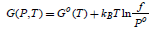
where f coincides with P. The parameter f is called the gas fugacity and represents the gas effective pressure and accounts for the non-idealness of the gas. It is convenient to introduce the so-called fugacity coefficient defined as

which shows that the Gibbs energy of the real gas can be formally seen as the corrected Gibbs energy of the ideal gas. Gnonid (P,T) depends directly on T and indirect on P through
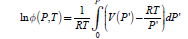
Thus the Gibbs energy of the gas can be calculated if the dependence V(P) is known from the equation of state and it can be treated within the mathematical framework of ideal gas thermodynamics.
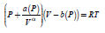
More accurate thermodynamic calculations especially at high pressures and at low temperatures can be done using the Van der Waals Equation of State.[56] At ambient temperature (298.15 K) the pressure of the real gas vs. molar volume can be described by
where:
- p is the gas pressure,
- V the volume occupied by one mole of gas,
- T the absolute temperature,
- R the gas constant,
- a is the dipole interaction or repulsion constant,
- b is the volume occupied by the gas molecules.
For the hydrogen molecular gas, a has the value 2.476102 m6·Pa·mol-2 and b = 2.661105 m3·mol-1 [57]. The parameter a describes the strong repulsion interaction between hydrogen molecules and it is responsible for the low critical temperature (Tc=33 K) of hydrogen gas. For low pressures the Van der Waals correction does not significantly change the dependence G(P,T) for the molecular hydrogen gas, comparing to the ideal-gas model. Several other forms of the EOS are proposed for hydrogen and its isotopes [58].
An elegant formulation starts from the Van der Waals equation of states is the Peng−Robinson EOS, where, where the coefficients a(T) and b(T) are temperature-dependent [59]. An alternative EOS treat the coefficients a(P) and b(P) are considered depending on pressure and the α(T) exponent as depending on temperature [60]
where
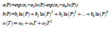
The values of the parameters ai, bi and αi for the molecular hydrogen fluid are given in the Table S3.
Table S3: The parameters ai, bi and αi of the generalized Van der Waals equation of state [60]

For an isothermal transformation, the variations of the thermodynamics parameters are
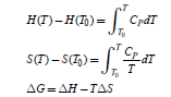
where T0 is usually considered the standard temperature of 298.15 K. Thus, the Shomate equation [61] that gives the temperature dependence of the Gibbs free energy at Po

can be obtained.
Table S4: The parameters A-F in the Shomate equation of the standard Gibbs energy (given in J/mol H2) for a temperature in the range 273 - 1000 K for the molecular hydrogen. [62-64]

Below and around the reference pressure Po the Gibbs free energy can be calculated using the ideal gas model as Go (T)Gid (T) . Considering the compressibility of the gas Joubert [65] proposed for the non-ideal component of the Gibbs free energy a pressure dependency as
The values of the ai, bi, c, and d coefficients (see Table S5) for the molecular hydrogen gas are determined by the fit of the experimental data.
Table S5: The values of the parameters that give the pressure dependence of the Gibbs energy of the fluid hydrogen [65].

Thus the P and T dependency of the Gibbs free energy within the real gas model can be completely estimated in the frame of the CALPHAD method. As the ideal component of the Gibbs free energy can be calculated based on the thermodynamic calculations based on the DFT method, just Gnonid (P) has to be calculated by the Joubert scheme [65]. Thus the boundary curve for the formation and decomposition of the magnesium hydride can be determined by the thermodynamic calculations based on the DFT electronic structure method.
References
- Errandonea D, Meng Y, Häusermann D, Uchida T (2003) J Phys Condens Matter 15: 1277.
- Perez-Albuerne EA, Clendemen RL, Lynch RW, Drickamer HG (1966) Phys Rev 142: 392.
- Errandonea D (2004) J Phys Condens Matter 16 8795 (Replay to [4]).
- Olijnyk H (2004) J Phys Condens Matter 16 8791 (Comments on [1]); Yao Y, Klug D (2012) J Phys Condens. Matter 24: 265401.
- Li P, Gao G, Wang Y, Ma Y (2010) J Phys Chem C 114: 21745.
- JA Moriarty and JD Althoff (1995) Phys Rev B 51: 5609.
- D Errandonea, R Boehler, and M Ross (2001) Phys Rev B 65: 012108.
- P Toulemonde, C Goujon, L Laverssene, P Bordet, R Bruyere, M Legendre, et al. (2014) High Press Res 34 167.
- Errandonea DY Meng, D Häusermann and T Uchida (2003) J Phys Condens Matter 15: 1277.
- J Xiao, R Li and Y Wu TMS (2015) Annual Meeting Supplemental Proceedings, (The Minerals, Metals & Materials Society p. 1379.
- M Pozzo and D Alfè (2008) Phys Rev B 77:104103.
- EY Tonkov and EG Ponyatovsky (2005) “Phase Transformations of Elements under High Pressure”, (CRC Press: p. 44.
- H Olijnyk and WB Holzapfel (1985) Phys Rev B 31: 4682.
- G Colonna, A D’Angola and M Capitelli (2012) Int J Hydrogen En 37: 9656.
- JW Leachman, RT Jacobsen, SG Penoncello and EW Lemmon (2009) J Phys Chem Ref Data 38: 721.
- N Sakoda, K Shindo, K Shinzato, M Kohno, Y Takata and M Fujii (2010) Int J Thermophys 31: 276.
- YA Çengel, JM Cimbala and RH Turner (2017) “Fundamentals of thermal-fluid sciences”, 5th Ed (McGraw-Hill Education: Boston, p. 112.
- FE Simon and G Glatzel, Z Anorg (1929) (Allg) Chem 178: 309.
- V Diatschenko and CW Chu (1981) Science, 212: 1393.
- VV Kechin (1995) J Phys Condens Matter 7: 531.
- F Datchi, P Loubeyre and R LeToullec (2000) Phys Rev B 61: 6535.
- S Scandalo, Proc Natl Acad Sci USA, 100 (2003) 3051; SA Bonev, E Schwegler, T Ogitsu and G Galli, Nature (London), 431 (2004) 669; SM Davis, AB Belonoshko, B Johansson, NV Skorodumova, and ACT van Duin, J Chem Phys 129 (2008) 194508; MA Morales, C Pierleoni, E Schwegler, and DM Ceperley, Proc Natl Acad Sci U.S.A 107 (2010) 12799; L Caillabet, S Mazevet, and P Loubeyre (2011) Phys Rev B 83: 094101; A. B. Belonoshko, M. Ramzan, H. K. Mao, and R. Ahuja, Sci. Rep 3 (2013) 2340; HY Liu, ER Hernandez, J Yan, and YM Ma (2013) J Phys Chem C 117: 11873.
- MI Eremets and IA Trojan (2009) JETP Lett 89: 174.
- E Gregoryanz, AF Goncharov, K Matsuishi, H Mao, and RJ Hemley (2003) Phys Rev Lett 90: 175701; S Deemyad and IF Silvera (2008) Phys Rev B 100: 155701; N Subramanian, AF Goncharov, VV Struzhkin, M Somayazulu, and RJ Hemley (2011) Proc Natl Acad Sci USA 108: 6014.
- I Silvera (2010) PNAS, 107: 12743.
- JM McMahon, MA Morales, C Pierleoni and DM Ceperley (2012) Rev Mod Phys 84: 1607; IB Magdau, M Marques, B Borgulya and GJ Ackland (2017) Phys Rev B 95: 094107; IB Magdau, F Balm and GJ Ackland (2017) J. Phys Conf Series 950: 042059.
- HK Mao and RJ Hemley (1994) Rev Modern Phys 66: 671; RT Howie, CL Guillaume, T Scheler, AF Goncharov and E Gregoryanz (2012) Phys Rev Lett 108: 125501.
- J Chen, X Ren, XZ Li, D Alfè and E Wang (2014) J Chem Phys 141: 024501.
- NIST Reference Fluid Thermodynamic and Transport Properties Database (REFPROP): Version 8.0, http://www.nist.gov/srd/nist23.htm; https://h2tools.org/hyarc/hydrogen-data/hydrogen-density-different-temperatures-and-pressures.
- M J Moran and HN Shapiro (2006) “Fundamentals of Engineering Thermodynamics”, 5th Ed (John Wiley & Sons Ltd p. 96.
- EW Lemmon, ML Huber and JW Leachman (2008) J Res Natl Inst Stand Technol 113341; www.nist.gov/publications/revised-standardized-equation-hydrogen-gas-densities-fuel-consumption-applications.
- H Hemmes, A Driessen and R Griessen (1986) J Phys C Solid State Phys 19: 3571.
- EW Lemmon, ML Huber and JW Leachman (2008) J Res Natl Inst Stand Technol 113: 341; www.nist.gov/publications/revised-standardized-equation-hydrogen-gas-densities-fuel-consumption-applications.
- FD Rossini (1970) J Chem Thermod 2: 447.
- P Lasgorceix and MA Dudeck (1991) Exp Therm Fluid Sci 4: 301; W Ebeling, WD Kraeft and D Kremp (1986) Europhys News 17: 52; B Militzer, W Magro and D Ceperley (1999) Contrib. Plasma Phys 39: 151.
- AlY Potekhin, G Chabrier and YA Shibanov (2000) Phys Rev E 60: 2193; ibid 63: 019901.
- S Scandolo (2003) PNAS, 100 3051; MA Morales, C Pierleoni, E Schwegler and DM Ceperley (2010) PNAS, 107 12799; MA Morales, JM McMahon, C Pierleoni and DM Ceperley (2013) Phys Rev Let 110” 065702; C Pierleoni, MA Morales, G Rillo, M Holzmann and DM Ceperley (2016) PNAS, 113: 4953.
- V Dzyabura, M Zaghoo and IF. Silvera (2013) PNAS 110: 8040.
- M Rossh, C Graboske, WJ Nellis, Phil Trun r. R (1981) Soc Land A303 303; ST Weir, AC Mitchell and WJ Nellis Phys Rev Lett 76 (1996) 1860; WJ Nellis, Chem Eur J 3 (1997) 1921; MI Eremets and IA Troyan (2011) Nature Mat10: 927.
- SR Bahn and KW Jacobsen (2002) Comput Sci Eng 4: 56; AH Larsen et al (2017) J Phys Condens Matter 29: 273002; https://wiki.fysik.dtu.dk/ase/.
- https://wiki.fysik.dtu.dk/ase/ase/thermochemistry/thermochemistry.html.
- M Valiev, EJ Bylaska, N Govind, K Kowalski, TP Straatsma, HJJvan Dam, D Wang, J Nieplocha, E Apra, TL Windus and WA de Jong (2010) Comput Phys Commun 181: 1477; http://www.nwchem-sw.org.
- GJ Martyna and ME Tuckerman (1999) J Chem Phys 110: 2810.
- AD McLean, A Weiss and M Yoshimine (1960) Rev. Mod. Phys 32: 211.
- BP Stoicheff, Can (1957) J. Phys 35: 730.
- KP Huber and G Herzberg (1979) “Molecular Spectra and Molecular Structure IV. Constants of Diatomic Molecules”, (Springer Science and Business Media: New York, p. 240.
- BP Stoicheff (1957) Can J Phys 35: 730.
- GD Dickenson, ML Niu, EJ Salumbides, Komasa J, KSE Eikema, K Pachucki and W Ubachs (2013) Phys Rev Lett 110: 193601.
- http://www.cup.uni-muenchen.de/ch/compchem/vib/vib1.html (accessed July 2018).
- IM Alecu, J Zheng, Y Zhao, and DG Truhlar (2010) J Chem Theory Comput 6: 2872.
- M Tkacz and A Litwiniuk (2002) J Alloys Compd 89: 330.
- Donald Allan McQuarrie (1976) Statistical Mechanics (HarperCollins, page 228
- P Fu, R Jia, CP Kong, RI Eglitis and HX Zhang (2015) Int. J. Hydrogen En 40: 10908.
- K Patkowski, W Cencek, P Jankowski, K Szalewicz, JB Mehl, G Garberoglio and AH Harvey (2008) J Chem Phys 129: 094304; G Garberoglio, P Jankowski, K Szalewicz AH (2012) Harvey J Chem Phys 137: 154308.
- P Perrot, “A to Z of Thermodynamics”, (Oxford University Press, 1998), p. 120.
- A Zuttel Naturwissenschaften (2004) 91: 157.
- “Handbook of chemistry and physics” (1976) 57th edn Ed.: Weast, (CRC, Boca Raton).
- M Tkacz and A Litwiniuk (2002) J. Alloys Compd 330–332: 89.
- Peng and DB Robinson (1976) Ind. Eng. Chem. Fundam 15 59; V. Vinš and J. Hruby (2011) Int. J. Refrig 34: 2109.
- H Hemmes, A Driessen, R Griessen (1986) J Phys C 19: 3571.
- CH Shomate (1944) J Am Chem Soc 66: 928.
- AT Dinsdale (1991) CALPHAD, 5: 317.
- MW Chase Jr CA Davies, JR Downey Jr DJ Frurip, RA McDonald, AN Syverud (1985) “Third edition of JANAF thermochemical tables”, J. Phys. Chem. Ref. Data (Suppl. 1): 100; M. W. Chase, , Jr “NIST-JANAF Themochemical Tables” (1998) 4th Ed J. Phys. Chem. Ref. Data, (Monograph 9), 1.
- MW Chase (1998) S NIST-JANAF thermochemical tables, 4th Ed J. Phys. Chem. Ref. Data, (Monograph 9),; https://janaf.nist.gov/
- JM Joubert A (2010) Int. J. Hydrogen En 35 2104.


-

Mark E Smith
Bio chemistry
University of Texas Medical Branch, USA -

Lawrence A Presley
Department of Criminal Justice
Liberty University, USA -

Thomas W Miller
Department of Psychiatry
University of Kentucky, USA -

Gjumrakch Aliev
Department of Medicine
Gally International Biomedical Research & Consulting LLC, USA -

Christopher Bryant
Department of Urbanisation and Agricultural
Montreal university, USA -

Robert William Frare
Oral & Maxillofacial Pathology
New York University, USA -

Rudolph Modesto Navari
Gastroenterology and Hepatology
University of Alabama, UK -

Andrew Hague
Department of Medicine
Universities of Bradford, UK -

George Gregory Buttigieg
Maltese College of Obstetrics and Gynaecology, Europe -

Chen-Hsiung Yeh
Oncology
Circulogene Theranostics, England -
.png)
Emilio Bucio-Carrillo
Radiation Chemistry
National University of Mexico, USA -
.jpg)
Casey J Grenier
Analytical Chemistry
Wentworth Institute of Technology, USA -

Hany Atalah
Minimally Invasive Surgery
Mercer University school of Medicine, USA -

Abu-Hussein Muhamad
Pediatric Dentistry
University of Athens , Greece
