Prediction of SPM Concentration Using Air Dispersion Model: A Case Study of Thermal Power Plant Volume 6 - Issue 1

Akshey Bhargava¹*, Megha TS² and SheetalKamble³

• ¹Ex. Rajasthan Pollution Control Board, CEPT University, India
• ²Department of Civil Engineering (Translational Engineering), Government Engineering College Barton Hill, India
• ³Assistant Professor, Environmental Science, P P Savani University, India

Received: February 04, 2021   Published: February 24, 2021

Corresponding author: Akshey Bhargava, Ex. Rajasthan Pollution Control Board, CEPT University, India

DOI: 10.32474/OAJESS.2021.06.000229

Abstract PDF

Air pollution has been termed as a democratizing force, but it is far from that, as it propagates existing environmental injustices. Industrial development and rapid urbanization have adversely affected urban air quality due to industrial and vehicular emissions. Air pollution exposure has shown to affect cognitive development in children, slow lung development and has resulted in high levels of mortality from respiratory infections. The elderly is more likely to develop cardiac illnesses and chronic respiratory as a result of long-term exposure and are more susceptible to strokes and heart attacks during episodic high pollution events. Thermal Power Plant has been a major source of air pollution for so long. Increasing health problems has made particulate matter to give special attention by control technology and framing regulations. Suspended particulate matter (SPM) is considered to be the main pollutant emitted by the power station. Atmospheric dispersion pollution modelling is of great and actual concern in the scientific international community. Many dispersion models have been developed and used to estimate the downwind ambient concentration of air pollutants from sources such as industrial plants, vehicular traffic, or accidental chemical release. Among them, Gaussian model is perhaps the most commonly used model type. It is often used to predict the dispersion of air pollution plumes originated from ground-level or elevated sources. An attempt has been made in the present paper by the authors to discuss such models with a view to select a particular model that can be used for a particular area or application. An effort has also been made to predict SPM concentrations from a coal based thermal power plant at various receptor points using model of Gaussian dispersion.

Keywords: Suspended particulate matter (SPM); Thermal power plant; Air dispersion model; Gaussian approach; Dispersion coefficients; Predictions; Urbanization; Gaussian model; Atmospheric dispersion modelling; Meteorology; Mitigation; Air pollution; Turbulent fluxes; Atmosphere; Estimated wind velocities

The dispersion of air pollution both in urban areas and open spaces is becoming of great concern in the scientific community. The concern for air quality has been an issue with Indian government for the past few years. Growing urbanization along with industrial and vehicular pollution is leading to environmental degradation faster than in other countries. A thriving industrial base and rapid economic growth–about 5% a year–account for much of the severe pollution, which costs India an estimated $9.7 billion a year in environmental damage. In last decades, the normal levels of air pollution have increased [1] and many countries have started to focus to develop monitoring systems for air pollution. Air quality models are able to predict the pollutant gases or aerosol trajectories in atmosphere. The evaluation and calibration of dispersion models is of a crucial importance, because their results often influence decisions that have large public-health and economic consequences. Obviously, there are different types of models and their performances depend on many variables. The classification of these models may refer about the source type (point source, line source, and area source), the adopted scale (large or small scale), the input type (deterministic models and stochastic models), the dynamic conditions (steady or unsteady state), and the pollutant sources (gases or particles). Among them, Gaussian model is perhaps the most commonly used model type. These are widely used in atmospheric dispersion modelling, usually in regulatory purposes because of their easy implementation and their near realtime responds. They generally are used in large scale applications [2]. Suspended particulate matter (SPM) levels in the air have been found to be at critical levels in urban cities, especially in residential areas, in India. The ambient levels of SPM in most of the urban areas of India are above 150mg/m3, which far exceeds the WHO standards of 50mg/m3 [3]. The coal-based thermal power plants, constitute 62.3% of electric power generation, are considered to be one of the chief industrial emitters of SPM in India. Increasing reliance on coal as the main fossil fuel in thermal power generation has led to numerous environmental problems [4]. Table 1 gives the share of coal and other fuels in electric generation along with the amount of SPM emitted per kilogram of fuels used.

Air pollution modelling is a numerical tool used to describe the causal relationship between emissions, meteorology, atmospheric concentrations, deposition, and other factors. This tool can give a complete deterministic description of the air quality problem, including an analysis of factors and causes (emission sources, meteorological processes, and physical and chemical changes), and some guidance on the implementation of mitigation measures [5]. One of the main challenges of atmospheric dispersion modelling is to develop models and software that can provide numerical predictions in an accurate and computationally efficient way. The concentrations of substances in the atmosphere are determined by 1) transport, 2) diffusion, 3) chemical transformation, and 4) ground deposition. The study of diffusion (turbulent motion) is more recent [5]. Chemical species such as NOx, SO2, which have longer lifetimes (hours-days) can have wider impact zones [6]. Therefore, in such cases regional or continental modelling approaches are needed. For simulating the dispersion of air pollutants, various modelling approaches have been developed. The application of air dispersion models [7] are quite wide in as much as that it is effectively used for urban planning, industrial estate planning, industrial zoning, sitting of industrial project and overall special planning from environmental point of view. Modelling can be used to analyze actual or potential accidents that release contaminants to the atmosphere. Other applications are as under:

1. Assessing compliance of emissions with air quality guidelines, criteria, and standards
2. Planning new facilities
3. Determining appropriate stack heights
4. Managing existing emissions
5. Designing ambient air monitoring networks
6. Identifying the main contributors to existing air pollution problems
7. Evaluating policy and mitigation strategies (e.g., the effect of emission standards) forecasting pollution episodes
8. Assessing the risks of and planning for the management of rare events such as accidental hazardous substance releases
9. Estimating the influence of geophysical factors on dispersion (e.g., terrain elevation, presence of water bodies and land use)
10. Running ‘numerical laboratories’ for scientific research involving experiments that would otherwise be too costly in the real world (e.g., tracking accidental hazardous substance releases)
11. Saving cost and time over monitoring – modelling costs are a fraction of monitoring costs and a simulation of annual or multi-year periods may only take a few weeks to assess.

Types of Air Dispersion Models

Air pollution models can be categorized into three generic classes: deterministic approach, statistical models, and physical models. Deterministic models basically deal with different types of numerical approximations (for example finite difference and finite techniques) in the solution of the partial equations representing the relevant physical process of atmospheric dispersion. The deterministic model is most suitable for long-term planning decisions. In contrast to the deterministic model, the statistical one calculates ambient air concentrations using an empirical established statistical relationship between meteorological and other parameters on the other hand [8]. The statistical model is very useful for short-term forecast of concentrations. In physical models, a real process is simulated on a smaller scale in the laboratory by a physical experiment, which models the important features of the original process being studied. The most important advantage of physical models is that the scale-model geometry, as well as flow speed and other essential variables can be easily changed and controlled [8].

Deterministic model

Most of the deterministic model use or are equivalent to using solutions of the diffusion equation. The diffusion equation is based on the principle of conservation of mass. The turbulent fluxes of material are expressed by the gradient relationship, i.e., it is assumed that the turbulent flux is proportional to the gradient of concentration and the proportionality ‘constant’ is called the diffusion coefficient. The diffusion equation reads as follows:

The symbols have following measuring:
c = the time – averaged concentration
x, y, z = the Cartesian coordinates
u, v, w = the components of the time-averaged wind vector
k_x, k_Y, k_Z = the diffusion coefficient in the corresponding direction
The boundary condition at the earth’s surface has to be stated and it is often assumed that the diffusing material (gases) is not absorbed by the ground, i.e., the material is ‘reflected’ into the atmosphere. The other extreme case that all material reaching the surface is absorbed, is not appropriate, at least not for gases. Partial reflection of the material at the ground is the most realistic case, but it involves the statement of another parameter, which is usually called the deposited velocity. Often a boundary condition for the upper boundary of the diffusion volume is stated, especially in case of an inversion [8]. In that case, too, the total reflection assumption at the upper boundary is used. The models calculate the concentration at one receptor point from one source. If more than one source is present, then the contributions from each source at the receptor point are summed.

Gaussian plume model

The greatest advantage of Gaussian Plume models is that they have an extremely fast, almost immediate response time. Their calculation is based only on solving a single formula for every receptor point, and the model’s computational cost mainly consists of meteorological data pre-processing and turbulence parameterization. Depending on the complexity of these submodules, the model’s runtime can be extremely reduced enabling its application in real-time and near real-time decision support software [9]. Gaussian dispersion models have become a uniquely efficient tool of air quality management for the past decades, especially in the early years when high performance computers had an unreachable price for environmental protection organizations and authorities. Their fast responds depend basically on several assumptions that make them useful for just some applications. The main important assumptions are:
a) The emission rate of the source is constant.
b) Dispersion (diffusion) is negligible in the downwind direction.
c) Horizontal meteorological conditions are homogeneous over the space modelled.
1. For each step modelled:
a. Wind speed is constant.
b. Wind direction is constant.
c. Temperature is constant.
d. Mixing height is constant.
e. No wind shear in the horizontal or vertical plane.
f. The pollutants are non-reactive gases or aerosol.
g. The plume is reflected at the surface with no deposition or reaction with the surface.
h. The dispersion in the crosswind and vertical direction takes the form of Gaussian distributions.
The sources types may be different: point source, volume source, area source, open pit and flare. Usually, it is possible to implement Gaussian models for more than one source and as assumption it is considered the Superposition principle.

An effort has been made in the present paper to develop air dispersion model by using Gaussian distribution approach. While developing this model, source strength of SPM based on composition of fuel has been estimated along with meteorological conditions were analyzed on Annual and seasonal basis to form a part of input data in the model. Similarly, plume rise from 10 model equations were estimated and the average value of the plume rise was considered in the present model. The atmospheric stability was also analyzed for making use in this model. The ground level concentrations of SPM were estimated under all stability conditions starting from A to till category F. An isopleths were then prepared using surfer9 software. The predictions were done up to a distance of 120 km from the Gandhinagar thermal power plant. The vertical and horizontal dispersion coefficients were estimated using following equations.

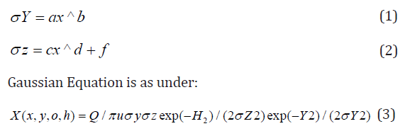
By using above equations and assuming constants as referred in above Tables 1 & 2, the values so obtained for σy and σz at various distances are as under (Tables 3 & 4). Subsequent to estimation of σy and σz under all atmospheric stability conditions, the wind velocity at stack heights of Gandhinagar thermal power plant were estimated using power law, the equation of which is as under.

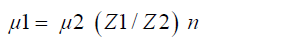
Table 1: Share of fuel in electric generation and emission per unit.

Table 2: Showing the values of constants {when x is < 1 km}(Wark and Warner, 1981).

Table 3: Showing the values of constants {when x is >1 km} (Wark and Warner, 1981).

Table 4: Showing values of σy under all stability conditions.

Where, μ1 and μ2 are wind speeds at height Z1 and Z2 respectively.
n is an exponent, is a function of stability class as shown in Table 5. Gandhinagar thermal power plant has five stacks attach to different units of power production; the details of each stack are as reflected in Table 6 below. The wind velocities at different stack heights indicated in Table 6 above were estimated using power law and values of exponent n referred in Table 4. The Average Estimated wind velocities at different stack heights under different stability conditions and directions for annual and different seasons are given in the following Tables 7-10. By using above equations and assuming constants as referred in above tables, the values so obtained for σy& σz at various distances are as under: Subsequent to estimation of σy&σz under all atmospheric stability conditions, the wind velocity at stack heights of Gandhinagar thermal power plant were estimated using power law , the equation of which is as under.

μ1= μ2 (Z1/Z2) n,

Table 5: Showing values of σz under all stability conditions.

Table 6: Showing the values of exponent “n”.

Table 7: Showing Stack Details of Gandhinagar Thermal Power Plant.

Table 8: Showing annual avg. wind velocity at different stack height.

Table 9: Showing Winter avg. wind velocity at different stack height.

Table 10: Showing summer avg. wind velocity at different stack height.

Where, μ₁, μ₂ are wind speeds at height Z1 & Z2 respectively. n is an exponent, is a function of stability class and is shown in Table 5 below. Gandhinagar thermal power plant has five stacks attach to different units of power production, the details of each stack are as under as per field monitoring and analysis. The wind velocities at different stack heights indicated in table above were estimated using power law and values of exponent n referred in Table 6. The Average Estimated wind velocities at different stack heights under different stability conditions and directions for annual and different seasons are calculated and given in the following tables. The values of average wind velocities at stack heights under different directions were used in the model as one of the input for predicting Annual average, winter, summer & Monsoon ground level concentrations of SPM at different receptor points. Similarly, as an input to air dispersion model, the source strength of SPM was also estimated using different methods However, the source strength considered in the model is given in the following table for different stacks. Similarly, plume rise was estimated using different model equations. The plume rise considered in the model is given in the following table .Having all the above parameters as an input to air dispersion model, the predicted concentration of SPM was estimated on annual and seasonal basis. The isopleths were also drawn in respect of SPM for different seasons & on annual basis under all the stability conditions. On the basis of predicted values, the isopleths for Annual SPM concentration have been drawn for all the stability conditions and some of them are being given in the Figures 1-7. Similarly, an effort has also been made to analyze the maximum concentration of predicted Annual SPM values in each direction under different stability condition at a particular distance. Such estimation has been shown in Tables 13 & 14. Similarly, Table 15 showing maximum predicted concentrations of SPM on annual, winter, summer, and monsoon seasons under all atmospheric stability conditions (A - F). It would be evident from above table that maximum predicted concentrations of SPM occur during winter season (54.64 μg/m³) followed by annual, monsoon and least in summer (9.73 μg/m³) under atmospheric stability A. It would also tend to show that maximum concentrations occur under stability A and the concentration decreases with the shifting of atmospheric stabilities from A to F.

Figure 1: Annual average predicted concentration of SPM under atmospheric stability A.

Figure 2: Annual average predicted concentration of SPM under atmospheric stability B.

Figure 3: Classification of Air quality Models (Modified from Weber, 1982).

Figure 4: Annual average predicted concentration of SPM under atmospheric stability C.

Figure 5: Annual average predicted concentration of SPM under atmospheric stability D.

Figure 6: Annual average predicted concentration of SPM under atmospheric stability E.

Figure 7: Annual average predicted concentration of SPM under atmospheric stability F.

Table 11: Showing Monsoon avg. wind velocity at different stack height.

Table 12: Showing source strength of SPM from different stacks.

Table 13: Showing plume rise from different stacks under different stability conditions.

Table 14: Showing maximum concentration of Annual SPM at a distance under each stability category under different directions.

Table 15: Showing maximum predicted concentrations of SPN under all seasons and atmospheric stabilities.

An effort has also been made to analyze the maximum concentration of predicted Annual SPM values in each direction under different stability condition at a particular distance. The findings are such estimations are shown in Table 14. It would be seen from Table 13 that the maximum annual average SPM concentration is 13.66 μg/m3 at a distance of 2 km under atmospheric stability A in ESE direction, followed by11.05, 10.53,9.37,8.93 & 7.80 μg/ m3 in SSE,NNE,SSW,NNW,ENE directions respectively but all at a distance of 2 km. Similarly, under atmospheric stability B, maximum concentration of SPM is of the order of 148.55 μg/m3 at a distance of 4 km, followed by 84.88,12.49,10.33,9.30 & 9.25 μg/m3 in ENE,SSE,NNE, SSW,NNW, directions respectively but all at a distance of 4 km. Moreover, under atmospheric stability c, maximum concentration of SPM is of the order of 131.62 μg/m3 at a distance of 8 km, followed by 75.21, 11.06, 9.15, 8.24 & 8.20 μg/m3 in ENE ,SSE,NNE,SSW,NNW directions respectively but all at a distance of 8 km. Similarly, under atmospheric stability D, maximum concentration of SPM is of the order of 27.196 μg/m3 at a distance of 52 km, followed by 15.54, 2.28, 1.89, 1.70& 1.69 μg/m3 in ENE, SSE, NNE, SSW, NNW directions respectively but all at a distance of 52 km. However, under atmospheric stability E, maximum concentration of SPM is of the order of 10.13 μg/m3 at a distance of 120 km, followed by, 5.78, 0.85, 0.70, 0.634& 0.631 μg/m3 in ENE, SSE, NNE, SSW, NNW directions respectively but all at a distance of 120 km. Similarly, under atmospheric stability F, maximum concentration of SPM is of the order of 2.51 μg/m3 at a distance of 120 km, followed by , 1.43,0.21,0.175,0.157 & 0.156 μg/ m3 in ENE ,SSE,NNE,SSW,NNW directions respectively but all at a distance of 120 km. From the above, it tends to indicate that under stability A , the maximum concentration occurs at a distance of 2 km whereas, this distance Increased to 4 km under stability B, 8 km under stability c, 52 km under stability D and 120 km under stability E & F. This analysis tends to show that the distance increases with shifting of stability from A to F. i.e., from highly unstable to highly stable conditions. Similarly, an attempt was also made to predict the ground level concentrations of SPM under all stability conditions for the season winter, summer, and monsoon. The Isopleths were also prepared but not being shown in the present paper due to huge volume. However, the Maximum predicted concentration of SPM under all stability conditions for all the seasons are shown in Tables 14 & 15.

Air pollution is growing on a rapid pace, not only in India but globally. It is becoming an emerging issue threating the health of human beings and environment as a whole. Air dispersion modeling is an important decision-making tool to predict air quality from air pollution sources on a scale of time and space. Such models are mandatory in the process of Environmental Impact Assessment and Management Plans required for environmental clearances. However, lot of research needs to be done for developing a scientifically compatible air dispersion models having regard to prevailing local conditions, reliable source strength, meteorological factors etc. Such studies need to be done on scale of time and space. Data base should be developed to keep all such research at one place for the benefit of other researchers.

1. Famoso F, Lanzafame R, Monforte P, Oliveri C, Scandura PF (2015) Air quality data for Catania: Analysis and investigation casestudy 2012-2013. Energy Procedia 81: 644-654.
2. Owen B, Edmunds HA, Carruthers DJ, Singles, RJ (2000) Prediction of total oxides of nitrogen and nitrogen dioxide concentrations in a large urban area using a new generation urban scale dispersion model with integral chemistry model. Atmospheric Environment 34(3): 397-406.
3. Sengupta I (2007) Regulation of suspended particulate matter (SPM) in Indian coal-based thermal power plants: A static approach. Energy Economics 29(3): 479-502.
4. Daly A, Zannetti P (2007) Air pollution modeling–An overview. Ambient air pollution pp. 15-28.
5. Leelőssy Á, Molnár F, Izsák F, Havasi Á, Lagzi I, and et al. (2014) Dispersion modeling of air pollutants in the atmosphere: a review. Central European Journal of Geosciences 6(3): 257-278.
6. Bhargava A, Patel P (2016) Air Dispersion Models for Different Applications - Special Reference to Thermal Power Plant. IJSDR 1(3): 121-124.
7. Srivastava S, Sinha IN (2004) March. Classification of air pollution dispersion models: a critical review. In Proceedings of National Seminar on Environmental Engineering with special emphasis on Mining Environment.
8. Brusca S, Famoso F, Lanzafame R, Mauro S, Garrano AMC and et al. (2016) Theoretical and experimental study of Gaussian Plume model in small scale system. Energy Procedia 101: 58-65.
9. Wark K, Warner CF (1981) Air Pollution Its Origin and Control.2nd Edition, Harper and Row Publishers, New York, USA.