Optimized Path Planning in Reinforcement Learning by Backtracking Volume 1 - Issue 4

Morteza Kiadi¹, Qing Tan²* and José R Villar¹

• ¹Computer Science Department, University of Oviedo, Spain
• ²School of Computing and Information Systems, Athabasca University, Athabasca, Canada

Received:June 28, 20199;   Published:July 26, 2019

*Corresponding author: Qing Tan, School of Computing and Information Systems, Athabasca University, 1 University Drive, Athabasca, AB, T9S 3A3, Canada

DOI: 10.32474/CTCSA.2019.01.000116

Abstract PDF

Abstract

Finding the shortest path to reach a destination in an indoor environment is so important that it is deemed as one of the fundamental and classical topics of Reinforcement Learning. Identifying the best path to reach a destination in a maze has been used as a testbed to learn and simulate Reinforcement Learning algorithms. In this paper, we developed a faster pathfinding model by optimization of the Markov decision-making process and tweaking the model’s hyper-parameters. The proposed method allows researchers to use the suggested optimized model in bigger state spaces. The presented results assist the researchers in this field to get a better idea of the Reinforcement Learning tenets and contributes to Reinforcement Learning community by making this topic more accessible. The problem we are going to solve it in the context of finding the shortest path in a smart lab “as soon as possible”. In this paper, we prove that the shortest path in a maze appears much sooner than finalizing the state values. By optimizing the code to behave smarter and extracting the recurrent visited states, we accelerate the search process to the magnitude of three times. Moreover, we compare the execution of the optimized codes on the dedicated cloud servers to simulate offloading the processing power from a robot to a more powerful processing server but in the proximity of the robot. This matter relates to the outcome of this paper to the Fog Computing in the context of robot pathfinding in indoor environments.

Keywords: Robot Path Planning; Reinforcement Learning; explore vs. exploit; Markov Decision Process; Smart Lab; Fog Computing

Introduction

There exist many solutions to the maze pathfinding problem for more than three decays. The problem is referred to as maze pathfinding, maze navigation, micro mouse and indoor robot pathfinding. Equally, there are different solutions to solve this problem through different method and algorithms. The Reinforcement Learning (RL) is one of the Machine Learning (ML) techniques that use trial and error to find an optimized solution to a problem [1]. The problem in this context is reaching a goal, like a specific location in an indoor environment. Despite the other machine learning techniques (i.e. supervised and unsupervised learning), it does not learn by labelled data. Instead, it learns by itself and performing an action and making decisions based on the feedback it receives from the environment. This feature makes the RL very different and to some extent, more unique compared to the other ML techniques. In RL, we do not specify “how” to achieve a goal, instead we rely on computation to find the best result. Therefore, finding a solution with less computation is one of the main research topics in RL. Reinforcement Learning has many applications in different scenarios such as cleaning robots, mining robots, and rescue robots [2].

This paper focuses on finding the shortest path in a controlled indoor environment, called “smart lab”. This study proposes a faster pathfinding model based on optimizing the decision-making process and fitting the hyper-parameters. At the same time, the study includes a comparison of performing the path planning on the robot through fog computing. The solution components are designed around the four main subcomponents of the reinforcement learning systems [1]: policy, reward signal, value function, and model. Furthermore, it consists of an agent, the environment to interact with and the goal to reach. After constructing the components and presenting the solution, we briefly discuss the exploit vs. explore dilemma in the RL. The explore and exploit do not exist in other machine learning methods. At the end of this paper, we have presented the results of our tests and optimization. We also compare our results after optimization. The solution is driven by a series of hyper parameters that we have explained and tweaked them before analyzing the results.

The structure of this paper is as follows. The next section details the related work in path planning. Section III introduces the problem of pathfinding in the smart lab and the pre-established assumptions. In Section IV we elaborate the solution components. After constructing the components and presenting the solution, we briefly discuss the exploit vs. explore dilemma in the section V. In the hyperparameters section VI, we have shown the parameters of the model that impact the performance and convergence time. In the optimization section VII of this paper, we explain the way we can improve the convergence time to find the optimal path. In the discussion section VIII, we have briefly compared our model with other models and finally, in the conclusion section, we will discuss the findings.

Related Work

The robot navigation in an environment is not a new topic and as a result, there exists great progress in this field. Instances are Kalman Filtering (EKF) to implement Simultaneous Localization and Mapping (SLAM) in a robot navigation task [3]. IEEE has established a set of rule solving the maze problem and launched a competition named “Micro mouse” [4] where an autonomous robot or mice solves an unknown maze. The micro mouse problem has been solved by different algorithms, including artificial intelligence and graph theories. Many researchers have modelled the problem of finding the shortest path in a maze in the form of a graph where the vertices are the cells and the edges are the feasible paths between those cells. Different graph theories like Breath First Search (BFS), Depth First Search (DFS) and its special version called Flooding are utilized to search the shortest path in a graph. Among many existing results, [5] has proved that the maze structure can change the performance of BFS and DFS. For example, DFS tends to explore all the cells in the graph that may be a big waste. DFS also needs more memory as this is the case for Flooding, in which it is a concern in mazes larger than 8x8.

In addition to the above-mentioned graph-based methods, other algorithms like A* and D* [6] [7] are suggested for the robot path planning and it is proved that A* overperform D* algorithm. The study in [8] in regard to the greedy DFS, has been proposed in path selection. [9] suggests a neural network to navigate a robot in an obstacle avoidance model based on multiple neural networks cooperation. In this case, the robot will be trained to make decisions based on the existing patterns. For example [10] has suggested a solution to navigate the robot to avoid collision and deciding based on 256 patterns. In this case, the 256 patterns are generated from 8 sonar reading that model the entire possible scenarios and off-line trained and learned by the artificial neural network.

Moreover, [11] proves that the Dijkstra algorithm can solve the maze robot path planning. The study in [12] has proposed a model to map the whole maze as a graph in standard “Adjacency-list representation” and finding the shortest path in the shortest time path by Dijkstra algorithm.

Recent advances in image processing and artificial intelligence has been utilized to build smarter robots in the maze. For example, authors in [13] have used an intelligent maze solving robot that can determine its shortest path on a line maze based on image processing and artificial intelligence algorithms. The image of the line maze is captured by a camera and sent to the computer to be analyzed and processed by a program and based on graph theory algorithms. The developed program solves the captured lines by examining all possible paths (hence supervised learning) in the maze that could convey the robot to the required destination point. The best shortest path is instructed to the robot to reach its desired destination point through Bluetooth. The authors in [13] have claimed that the solution works faster than the traditional methods which push the robot to move through the maze cell by cell in order to find its destination point. The research in [14] has solved the maze by upgrading the line maze solving algorithm (an algorithm used to solve a maze made of lines to be traced by a mobile robot) by using the curved and zigzag turns.

Others have solved the same problem by a combination of Zigbee wireless robots with markers in an indoor environment with a camera, image process and BFS and DFS algorithms for trajectory calculation, path planning and trajectory execution within an indoor maze environment [15]. The Lee algorithm [16] is used to find the shortest path in a maze that is implemented with a breadth-first search. The Maze is effectively “flooded with water”, and each point in the Maze keeps track of which direction it was flooded from.

The Smart Lab Problem

In general, the RL problem is about finding a series of actions that result in some best output. The mapping between all those actions to all the states that give the best result is captured in the form of a function called policy (ℼ) function. Hence, we are looking for the best ℼ, or optimal ℼ (ℼ*) in this context. The mapping function ℼ maps a state to an action, i.e. ℼ: SA and the job of RL is to find ℼ*. We can find ℼ* in two general ways: by “searching” the solution space and trying all possible scenario before choosing the best one or by “estimating” a function (function approximation) that generates the values. In this paper, we focus on the former approach since our assumptions around solving the smart lab problem are constructed around the following assumptions:

I. The reward signal of doing an action in the smart lab environment is static (we always give -1 for each move that is not resulted in reaching the target state). This assumption rolls out the idea of having stochastic rewards.

II. We do not allow our agent to move to an obstacle since the entire state space is observable and modelled. Having a model allows the agent to “plan” before moving.

III. The result of our action is not stochastic, and we do not need to use statistical techniques in solving the problem. IV. The state space is not too big and is not continuous. This assumption allows us to explore all the states in a space and make use of that in the planning.

V. The state space does not have any other moving object than the learner agent. That means the agent is the only moving object in the state space (i.e. we do not have a multi-agent environment).

VI. The state values that we would like to learn is the criteria to find the best path.

VII. We simulate the state environment in the form of a maze and try to find the best path in an offline manner (i.e. the robot would not move until the program finish its planning). In the context of robot path planning, this approach is called “global path planning”. In this paper, we did not assume that the robot has any sensory data and as a result, there is no real-time path planning (local path planning)

VIII. Since there is a model of the environment in the form of a maze, we can safely assume that the robot has the map

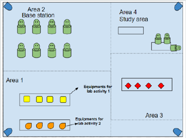
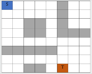
In the smart lab, there are obstacles like tables or chairs and surrounding walls. A robot has to move from a base station (start point) toward a target location in the lab, such as a table. The decisions that the agent makes depends on the topology and the environment model [17]. The topology of the environment is known ahead of time shown in [Figure 1]. The robot knows where the start location is and where the robot is heading, the target location.

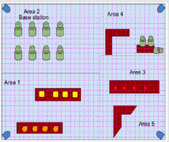
There are different ways to model and solve the movement of a robot in the lab such as using the graph theory techniques or computational geometry. In this paper, the solution method is based on modeling the indoor laboratory in the form of a grid or a maze shown in [Figure 2]. As a result, to solve this problem we abstract the problem statement to solve the robot movement from a cell in a grid from one cell to another cell. This scenario is very similar to one of the well research topics in the RL literature to move an agent in a maze (/grid). The agent is a software component that is given intelligence to make decisions sequentially based on the observations and the feedbacks that are received from the environment. The environment gives feedbacks to the agent about its last decision, in the form of immediate rewards (the primary reward). In addition to rewards, it presents the changes in the space state after performing the last action. In RL literature, this is called the state signal [1]. A maze is a simulation of a controlled environment where a robot (in which it carries the agent software) exists in it.

The Solution Components

In this section, we give details of the architecture and on how we found an optimal path before the search function is converged. In other words, instead of finding the best value in the states, we focus on finding the optimal route that appeared much sooner than the final value states.

A. Agent

An agent is a piece of software that is able to learn and take actions accordingly. It has the following features:

i. An agent has to be able to choose an action in a state

ii. An agent should know what is the best action to reach the goal. The agent does not know at the beginning and will learn about it gradually

“The best action” is formulated in the context of a dilemma in RL called “exploit vs. explore”. The agent has to explore new actions that are not identified necessarily as the best-learned action at the moment with this hope that it learns a new better way to achieve its goal. For example, 20% of the time it explores and 80% of the time it picks (exploits) the best action that has already learned. If the agent always exploits, then it uses what is called a “greedy” approach. The problem of the greedy approach is that it may never find the true best action. The agent has to learn from its actions.

Although there are more advanced methods such as Neural Networks (NN) to learn the best path to reach a destination from the existing data (for instance, existing robot navigation data), we have used a simple model in this paper. That is based on the reward system and the state value of the cell in the maze at each moment. Since the agent must learn from its actions, we should store state values in the form of a table, that is what we called state history table shown in [Table 1].

Every time a new episode is done, the state history table is updated.

Since the agent can learn, it should be able to keep track of and update its state history. In addition, the agent has to memorize the overall states it paves during learning, and it has to keep track of the steps it takes in each episode. This is important specifically in a multi-agent environment that the configuration of the state constantly changing due to other agents’ moves.

We should not confuse the state of the environment with the current state of the agent. For example at each point in time, the robot is in one specific state (position) in the entire state space. In our model, the only component that changes the state space is when the robot moves (the occupancy of the cells changes after each move). The agent must correlate its actions to the decisionmaking process. The glue between its actions and the decisionmaking process is the value of the states. We have covered this matter in the Future Reward section in this paper later.

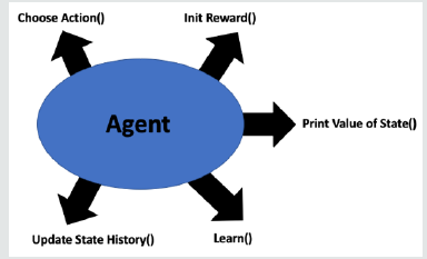
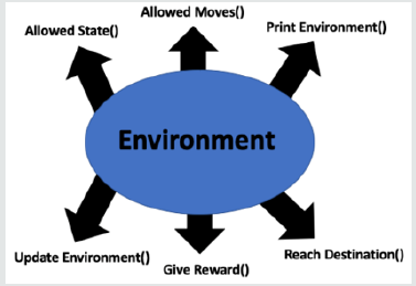
In the high level, the agent components have the functions we have described in [Figure 3].

<

B. Environment:

The environment is the “perception” of the agent about the world. We model the world for the agent in the form of its environment. It has the following features:

i. The environment at each point in time has a state. We let the agent observe that state.

ii. The agent’s moves can change parts of the state space but not all. For example, the state space’s free cells in the grid are changed when an agent moves from one state to another state (one cell is freed, and another one is occupied) but the obstacles are not changing. We need to keep track of the dynamic parts of the state space.

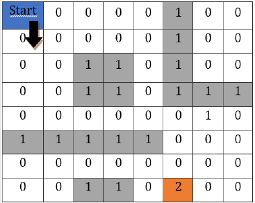
iii. We model the grid of the state space in the form of a matrix (an 8x8 matrix). We used the Python NumPy library for implementing the matrix. Each cell in the grid has one of the following statuses:

iv. It can be used by the agent and it is free now shown as an empty cell in [Figure 4] (value=0)

v. It cannot be occupied since it has an obstacle like a table or walls (value=1). Those are shown in grey color in [Figure 4] (a sample maze)

vi. It is the target cell that the robot is willing to reach (value=2)

By looking at [Figure 4], there are two obvious limitations in the agent’s moves:

a. The agent cannot move beyond the 8x8 grid

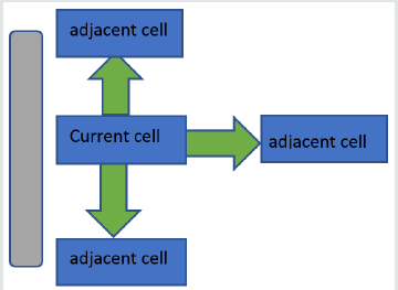
b. The agent cannot pass through the obstacles. As a result, we implemented a function to control the valid actions/moves in a cell based on the location of the agent and its immediately adjacent cells.

Our implementation includes a function to check if the robot has reached its destination (goal) after each move. Since we assumed to have only one agent in the environment (not being in a multi-agent environment) then nothing is going to change in the state space other than the state of the agent. In this case, it suffices to just track the state of the robot (the agent) in the state space. In the end, the environment would support the functions shown in [Figure 5].

C. Immediate Reward:

The reward indeed is a component that we could include it in the Environment section but we intentionally would like to discuss it separately to distinguish it from long-term rewards that we discuss it in the next section. The immediate reward is given to the agent based on the action that the agent has taken. If we do not have a proper rewarding mechanism, the entire RL will not work properly. In this research, we model a non-stochastic rewarding system based on the assumptions that the environment is static and only moving part is the robot. This static rewarding model rolls out the discussions around multi-arm bandit algorithms in our solution. The objective of the agent in its decision-making process is to maximize the reward it gets to take action. In this research, we did not include any other criteria other than maximizing the reward function. In the real world, usually there are more objectives to achieve such as reaching the goal with the objective of choosing the safest path (if there are more than one path to reach the destination), it is the shortest path and there is no collision with a moving obstacle.

A reward is a scalar value. We could give positive (+1) reward for any action that we consider them as “desirable” and give negative rewards ( -1) for the non-desirable actions. In our model, we just give (-1) for the actions that do not land the agent to the goal cell. The reward system should have the following features:

a. The reward mechanism should incentivize the agent to finish its task sooner

b. The above assumption enables us to enforce the agent to find the solution that is “optimized” than just finding a solution c. The above requirement means we need to give a negative reward for each step that does not lead to the goal state

d. The reward mechanism is not a prescription to solve the problem. It is simply a quantities measurement on the reward rate of action is in each step. It is the agent’s responsibility to find a solution.

D. Future Reward:

If there are three allowable moves for an agent to choose from in a state, for example, which move is the best action for the agent to pick to achieve the goal faster. The word “best” in this context is more or less a “time” factor in achieving the goal. It means that the agent should not only get to the destination but also reach the goal as soon as possible.

One way to solve this problem is to let the agent knows about the best action to pick in each state. In this case, there is no learning. The designer of the system programs the agent to pick the best action based on a logic that is programmed based on human judgment. Moreover, this approach is not scalable since the designer cannot predict all possible scenarios that may happen for a robot. Figure 6 shows how we can program an agent to always go down in being in a cell.

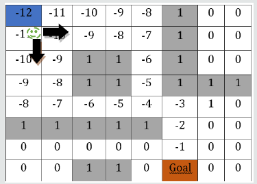
Humans can easily find the shortest path from an original location to a target location either by visual observation or by reverse path calculation, i.e. starting from the target and counting back to the start cell and accumulating (-1) reward in each step as it is shown in [Figure 7]. If we give the values of each cell to the agent as it is shown in [Figure 7], there is nothing to learn. The agent can simply look into its current neighbor’s cells values and choose either going down (-10) or right (-10) but surely not going up (-12). In this case, the agent picks an action that gives a lesser penalty, i.e. a greater reward. Our model was set to let the agent learns these values “by itself”.

It means that those negative values are the target values associated with each cell (cell values or state value). However, they are “unknown” to the agent in our model. The computation model helps the agent to learn those target values gradually by the trial and error. The function that helps the agent to learn those values is called “value function”. If the agent learns how to find the abovementioned values, then the agent has learned the best action to choose to reach the goal as fast as possible.

In the process of developing the model, the cells should be initialized with a random negative scalar. Those values are used in the learning process to calculate the above-mentioned target values. For example, if an agent has three valid moves, which move has to be selected? If the adjacent cells in Figure 8 have the same values, it is hard for the agent to select one over the others plus it takes longer time to converge since all the actions seem to have the same value at the beginning.

For that reason, the Python random function generates random values in the range of [-1,-0.1) for initialization of the cells. In this model since each cell has a different future reward, the agent will not be stuck in the middle of its operation. With each cell in the grid having a random value number, the agent needs to learn the best moves and “update” those values to help the agent to make a better decision in the next rounds.

In each round (or “episode”) the agent moves from the start point to the goal point. After each episode, the values of each cell has to be updated based on the agent’s selected path in that episode.

In our learning model, the state value of each cell is updated by formula 1. That is the “value function”. This formula calculates the gain value of a cell (G value). The gain values are nothing more than the state values in our model. That value of a cell helps the agent in its decision-making process. Our model tries to find the shortest path to reach the destination. The formula to update the value of each cell (the G value) after each episode is as follows:

In the model, we first initialized the entire state values by the Python random number generator to generate values between -1 and 0. We also set the target state value to 0 since there is no more gain to offer after reaching to the target cell.

In formula 1, the (target – existing G value of the state) is a way to calculate the error. The G value is a cell dependent value, i.e. each cell has its own value. So, in this case, our policy function (ℼ) selects the best move (up, down, right or left actions) based on the value of the states, if the idea is to exploit (not to explore).

The α is a parameter that we call it “learning rate”. It plays like a regulator in the formula. We have to find an appropriate value for this parameter and it is one of our hyperparameters to tweak in our experiment.

Exploit VS. Explore

When we know what actions are available in each cell (i.e. in each state), we must pick one of them that it gives the best gain in the longer term. What is the criterion to select the best action in each state? In our model, the criterion is the state value of the candidate cells to move to. We have to assign a value to each cell. The value shows the long term reward we get if we land on the cell. If we have 3 viable actions in a cell, each of those actions has a long term reward, associated with the cell values. We can simply select 80% of the time the best action and 20% of the time another random action. The 20%, in this case, is called “epsilon” and this method is called “epsilon-greedy”.

In the code, we initialize the ἑ -greedy value to 0.25. That means 25% of the time we choose a random action and 75% of the time we select the action in a cell that lands the robot to a cell with the best value. We anneal the epsilon in the course of learning to discount the exploration and increase the exploitation to calculate agent familiarity of the environment as time passes. The Epsilon is another hyperparameter that we tweaked in our optimization experiment.

Hyper-Parameters and Results

In the developed model, there are a few parameters that we have explored their impacts on the learning process.

We have summarized our findings in the following tables. The hyperparameters that we have explored are:

a. epsilon value in the ἑ -greedy

b. initial learning rate value (α)

c. Changes in the learning rate during execution (Annealing factor)

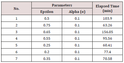
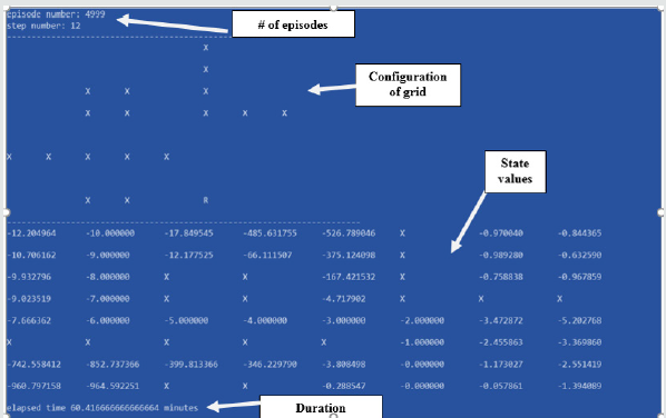
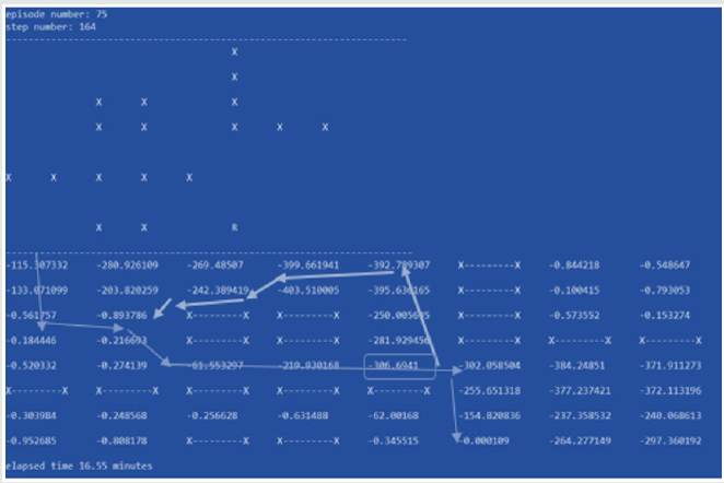
[Figure 9] illustrates one sample of the simulations. [Table 2] shows the best combination of epsilon (ἑ) and alpha () hyperparameters in our examination. It seems trial #5 (epsilon=0.25 and alpha=0.1) is an acceptable approximation for those hyperparameters. The configuration of the grid, the number of episodes, the values of the cells while learning was in progress and the elapsed times are shown in [Figure 9].

Initially, for an 8x8 maze, we set the number of episodes to a fixed number (3000 episodes). We observed that the final state values did not converge to the extent we wish. After increasing the number of episodes to 5000 episodes, we observed much better convergence as it is shown in [Figure 10].

However, waiting for almost half an hour to one hour to finish 5000 episodes for such a small state environment is not feasible in practice and it needs lots of computation. As a result, we have explored two optimization approaches inline with the hyperparameters in trial #5 mentioned in [Table 2].

Optimization by Backtracking

In the application to find the optimal path, we do not need to wait such a long time to calculate those precise state values. We proposed an optimization approach to find the optimized path by backtracking recurrence.

We are convinced that the optimal path can be found much sooner by monitoring the cells in a few consecutive iterations and stop if we observe the cells in consecutive episodes have recurred. By adding this idea to the logic, we experience 10 times improvement in the learning time.

In this section, the optimization approaches are going to be described and the results compared with other non-optimized iterations will be presented. To implement the optimization approach, the optimized code monitors the consecutive episodes and the steps that are used in those episodes to reach to destination and if they are identical, the process stops. Initially, we monitored two consecutive episodes however, we experienced a very edge case that two episodes in the initial episodes selected the same cells while the paved path was not an optimized path. To avoid this edge case, we decided to monitor three consecutive episodes and decide based on identicality of those three episodes.

For implementing the optimization code, two changes have to be applied. The code must store the track of the finished episodes and compare the result of each episode with the results of the last three episodes. These two processes add two steps in the execution of our code 1) writing the steps to a file, 2) comparing the last three episodes before starting the next episodes. Obviously, there is a performance penalty to introduce this I/O to the process, but this matter can be avoided to store the results in the memory instead of the disk. Although we have not implemented that, it is a way to make the code to find the optimized path even faster.

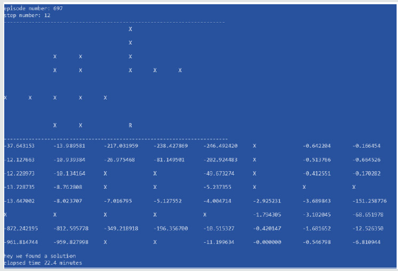
In an 8x8 maze, the elapsed time after optimization was 10 times faster or even better. It proves that it is a better approach and brings tremendous value, specifically in larger state spaces. As you see in Figure 11, the elapsed time is 22.4 minutes vs. 60.41 minutes (please see table 2, trial #5 that was the best value we got there) before optimization. The number of episodes is reduced to 697 episodes than 5000 episodes.

In our tests, the number of episodes has been decreased almost 7 times (5000 vs. 697 episodes) while the duration is decreased around 3 times (60.41 minutes vs. 22.4 minutes), which is because of the I/O that was introduced to the code.

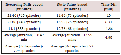
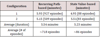
Another potential optimization is to change the code to investigate the state values (rather than looking for the recurred cells in episodes) and stop if the goal state value approximates the value 0.0. This approach made the pathfinding even process faster. [Figure 12] shows one instance of our experiment and the optimized path based on state values. We ran the optimized codes three times to get an average of time difference. The results are shown in [Table 3]. As it is shown, in our trials, on average the state-value based method saves around 5 minutes in an 8x8 maze while as it is true and expected that the state value optimization method outperforms, in situations, it falls behind the recurring path optimization methods (an example is the third instance of our experiment in table 3). This is more interesting when we compare the number of episodes in these two methods.

As it is illustrated in table 3, the number of episodes in the state value method has been decreased drastically (for example from 765 episodes to 73 episodes), almost 10 times less, while this is not true for the duration (i.e. we saved in times around 50%).

Discussion

The robot motion planning usually is decomposed to the path planning and trajectory planning. In path planning, we need to generate a collision-free path in an environment with obstacles and optimize it with respect to some given criteria [18]. If the environment is static, we can generate the path in advance (i.e. planning) and this is the approach we have chosen in this paper. As it is mentioned in the related work, there are many ways to solve the maze problem. Traditionally, there exist simple solutions for connected mazes. An instance of such simple solution is wallfollower (that sometimes it is called “left-hand rule “ or “the righthand rule”) by simply walking forward, keeping your left hand or right hand respectively on the wall at all times [19].

Many solutions, on the other hand, have chosen sensory data to discover the maze and make a decision in real time. Others have chosen to model the environment in the form of a grid and let the robot finds the shortest path by running different methods by utilizing the graph theory. When there is no real time sensory data, the pathfinding is done offline. The solution we have suggested in this paper learns the optimized path offline, but it did not use the graph theory. It tries to find the shortest path by comparing the last three episodes or monitoring the goal state value. We optimized the time by stopping the process when the path appears during the search process.

As it is shown in [Figure 12], at the point we have the state value -306.6941 (this state is shown in a rectangle in [Figure 9], the next better step is going up toward the state with the value of -281.92, while as we can see, that state actually moves the robot farther to the destination. This matter can be fixed by adding more logic to the code to identify the loops (that is more expensive to do) or to change the stop criteria to a more bigger number like (- 0.000001) to allow the learning process to continue for better results in the state values.

Another scenario that we did not include in this paper is multiagent environments. The main question in the multi-agent environments is how all other robots get each others’ updates. [20] has suggested each agent solve a part of the maze and update the shared memory so that other robots also benefit from each other’s’ discovery. Finding out the destination cell by an agent helps others to interconnect their discovered paths to the one ending with the destination cell. The proposed shortest path algorithm considers the cost for not only coordinate distance but also the number of turns and moves required to traverse the path. The Shortest Path algorithm is compared against various available maze solving algorithms including Flood-Fill and Modified Flood-Fill [A].

We have modelled the environment with a simple model to calculate the state values without using a sophisticated algorithmic approach. The model in this paper tries to find a good agent by finding a good state value. We have extended the results of [Table 3] by running the same two optimized codes on the cloud computing servers (i.e. offloading the processing to more powerful and dedicated devices) on two servers with the following configurations:

Configuration 1: 2 cores, 4 GB RAM

Configuration 2: 4 cores, 16 GB RAM

The result is shown in [Table 4]. As we can see, offloading the processing to more dedicated devices can improve the average pathfinding process in the recurring method from 18.47 minutes to 5.54 minutes. This improvement in the state value method is moving from 13.59 minutes to 5.23 minutes. This examination proves that we can gain around 3 times better performance with the above- mentioned configurations. We could use SSD and GPU processing in our configurations to even get better results.

Another interesting observation is that while the average # of episodes in the cloud servers for the recurring method compare to running the same method on the local laptop has not changed much (799 episodes vs. 718 episodes), the duration has been improved from 18.47 on average to 5.54 minutes). That speaks how much using fog computing in the proximity of the robots can improve the pathfinding process.

Another observation is that the state value method in the cloud server has taken more episodes (~ 86 episodes) than running it on the local laptop (72 episodes) while its execution time has been improved from 13.50 minutes in the local laptop to 5.23 minutes on the cloud servers. The increasing number of episodes proves the randomness of our experiments while the gained efficiency in the time on the cloud servers shows the significance of using fog computing servers

Conclusion

This research compared pathfinding durations in different settings such as different topologies, different epsilons, and different annealing factors. In addition, we showed two optimized methods to find the path by monitoring the recurring states and the state values as criteria to stop the episodes in the pathfinding process. The result of our experiments proved that generally, the state value monitoring has higher performance than the recurring state monitoring approach. This is not always the case but in the majority of cases that is proved to be true. We presented how the optimized path showed itself before concluding the 5000 episodes and how we can make use of this information in pathfinding in a shorter time.

The two optimization approaches mentioned in this paper need more exploration and improvements at least from the following two aspects:

A) Finding out the scenarios that state value optimization algorithm performs slower than the recurring value algorithm.

B) Finding out the best stop value criteria in the state-value optimization to avoid the loop.

C) Finding out the reason we have savings in the number of the episodes to the extent of 10 times less in the state value method compared with the recurring method while the gained saving in the time is around 50%.

We also showed how offloading the processing to more dedicated computing servers can improve the pathfinding process. The next step in the research is to compare the findings in this paper with state-of-the-art algorithms such as A*. In addition, such comparison can be conducted in the fog computing settings. The comparison can be done not only from the algorithmic perspective, but also from the constraint and the environment settings.

Acknowledgements

This research was conducted as a part of the research program: Telepresence Robot Empowered Smart Lab (TRESL) undergoing at Athabasca University. This research paper contributes to the first author’s PhD study at the University of Oviedo based on the MOU between the two universities. This research has been funded by the Spanish Ministry of Science and Innovation, under project MINECOTIN2017- 84804-R

References

1. R Sutton, A Barto (2018) Reinforcement learning: An Introduction 2nd ed The MIT Press 6-7
2. F Niroui, K Zhang, Z Kashino, G Nejat (2019) “Deep Reinforcement Learning Robot for Search and Rescue Applications: Exploration in Unknown Cluttered Environments,” IEEE Robotics and Automation Letters, 4(2) 610–617.
3. H Casarrubias Vargas, A Petrilli-Barcelo, E Bayro-Corrochano (2010) “EKF-SLAM and machine learning techniques for visual robot navigation,” 2010 International Conference on Pattern Recognition, Istanbul.
4. "Micromouse (2010) Competition Rules" IEEE Region 2 Student Activities Conference 2010 Web Page Web 21 Nov 2009.
5. A Sadik, M Dhali, H B Farid, T Rashid A Saeed (2010), "A Comprehensive and Comparative Study of Maze-Solving Techniques by Implementing Graph Theory", 2010 International Conference on Artificial Intelligence and Computational Intelligence.
6. X Liu (2011) “A comparative study of A-star algorithms for search and rescue in perfect maze,” 2011 International Conference on Electric Information and Control Engineering.
7. Takayuki Goto, Takeshi Kosaka, Hiroshi Noborio (2003) “On the Heuristics of A* or A Algorithm in ITS and Robot Path-Planning,” Proceedings of the 2003 IEEE/RSJ International Conference on Intelligent Robots and Systems. 1159-1166.
8. S Mahmud, U Sarker, M Islam, H Sarwar (2012) “A greedy approach in path selection for DFS based maze-map discovery algorithm for an autonomous robot,” 2012 15th International Conference on Computer and Information Technology (ICCIT). 546-550.
9. R del-Hoyo-Alonso, N Medrano-Marques, B Martin-del-Brio (2002) “A simple approach to robot navigation based on cooperative neural networks,” IEEE 2002 28th Annual Conference of the Industrial Electronics Society (IECON). 2421-2426.
10. K Chi, M R Lee (2011) "Obstacle avoidance in mobile robot using Neural Network," 2011 International Conference on Consumer Electronics, Communications and Networks (CECNet), Xian Ning. 5082-5085.
11. Huijuan Wang, Yuan Yu, Quanbo Yuan (2011) "Application of Dijkstra algorithm in robot path-planning," 2011 Second International Conference on Mechanic Automation and Control Engineering, Hohhot: 1067-1069.
12. S Sakib, A Chowdhury, S T Ahamed, S I Hasan (2014) "Maze solving algorithm for line following robot and derivation of linear path distance from nonlinear path," 16th Int'l Conf Computer and Information Technology, Khulna. 478-483.
13. M O A Aqel, A Issa, M Khdair, M El Habbash, M Abu Baker at el. (2017) "Intelligent Maze Solving Robot Based on Image Processing and Graph Theory Algorithms," 2017 International Conference on Promising Electronic Technologies (ICPET), Deir El-Balah. 48-53.
14. R J Musridho, F Yanto, H Haron, H Hasan (2018) "Improved Line Maze Solving Algorithm for Curved and Zig-zag Track," 2018 Seventh ICT International Student Project Conference (ICT-ISPC), Nakhonpathom.1-6.
15. S Jose, A Antony (2016) "Mobile robot remote path planning and motion control in a maze environment," 2016 IEEE International Conference on Engineering and Technology (ICETECH), Coimbatore. 207-209.
16. W Pullen (2016) "What is Lee Algorithm for maze routing problem?", www.quora.com.
17. Mishra, S and Bande, P (2008) Maze Solving Algorithms for Micro Mouse - IEEE Conference Publication [online] Ieeexploreieeeorg.
18. A Konar, I Goswami Chakraborty, S J Singh, L C Jain, A K Nagar (2013) "A Deterministic Improved Q-Learning for Path Planning of a Mobile Robot," in IEEE Transactions on Systems, Man, and Cybernetics: Systems, vol 43(5): 1141-1153.
19. B Gupta and S Sehgal (2014) "Survey on techniques used in Autonomous Maze Solving Robot," 2014 5th International Conference- The Next Generation Information Technology Summit (Confluence), Noida. 323-328.
20. B Rahnama, M C Özdemir, Y Kiran, A Elçi (2013) "Design and Implementation of a Novel Weighted Shortest Path Algorithm for Maze Solving Robots," 2013 IEEE 37th Annual Computer Software and Applications Conference Workshops, Japan. 328-332.