Complex Neural Fuzzy Prediction Using Multi-Swarm Continuous Ant Colony Optimization Volume 1 - Issue 3

Chunshien Li¹* and Wei-Chu Weng²

• ¹Department of Information Management, Nation Central University, Taiwan
• ²Department of Systems Engineering and Naval Architecture, National Taiwan Ocean University, Taiwan

Received:June 14, 2019;   Published:July 02, 2019

*Corresponding author: Chunshien Li, Department of Information Management, Nation Central University No. 300, Zhongli Taoyuan City 32001, Taiwan

DOI: 10.32474/CTCSA.2019.01.000115

Abstract PDF

Abstract

Prediction of time series is one of major research subjects in data science. This paper proposes a novel approach to the problem of multiple-target prediction. The proposed approach is mainly composed of three parts: the complex neuro-fuzzy system (CNFS) built by using complex fuzzy sets, the two-stage feature selection method for multiple targets, and the hybrid machine learning method that uses the multi-swarm continuous ant colony optimization (MCACO) and the recursive least squares estimation (RLSE). The CNFS predictive model is responsible for prediction after training. During the training of the model, the parameters are updated by the MCACO method and the RLSE method where the two methods work cooperatively to become one machine learning procedure. For the predictive model, complex fuzzy sets (CFSs) are with complex-valued membership degrees within the unit disk of the complex plane, useful to the non-linear mapping ability of the CNFS model for multiple target prediction. This CFS property is contrast to real-valued membership degrees in the unit interval [0,1] of traditional fuzzy sets. The two-stage feature selection applies to select significant features to be the inputs to the model for multiple target prediction. Experiments using real world data sets obtained from stock markets for the prediction of multiple targets have been conducted. With the results and performance comparison, the proposed approach has shown outstanding performance over other compared methods.

Keywords: Feature selection for multiple targets; Complex fuzzy set; Continuous ant colony optimization; Multiple swarms; Multiple target prediction

Introduction

Prediction of time series is one of major research subjects in data science. When data grows massively, effective prediction becomes much important. A novel approach is therefore proposed to effectively make multiple-targets prediction. It uses a complex neuro-fuzzy system where the involved parameters are decided by the proposed method MCACO-RLSE, integrating both the multiswarm continuous ant colony optimization (MCACO) algorithm and the well-known recursive least squares estimation (RLSE) method. In addition, a prediction system is developed to demonstrate the performance. The prediction system adopts a neuro-fuzzy system composed of several fuzzy if-then rules imbedded in neural network structure, where complex fuzzy sets and Takagi-Sugeno linear functions are used to define the premises and the consequents of rules, respectively. The adopted system is termed as Takagi-Sugeno complex neuro-fuzzy system (denoted as TS-CNFS in short). All parameters in the if-part are optimized by the method MCACO and those in the then-part are estimated by the method of RLSE. The method MCACO is a kind of continuous ant colony optimization (CACO) where multiple ant colonies are used. Furthermore, a twostage feature selection is applied to select the input data of the mostaffecting to multiple-targets. The method MCACORLSE associates two methods to decide all involved parameters separately and cooperatively. It comes out that the MCACO-RLSE helps the optimization effectively in the massively deflated solution space. The computation time is also decreased significantly. In addition, the two-stage feature selection presented in this paper selects only a few inputs to make multiple-targets prediction.

In the paper, practical stock prices and indices are chosen as case studies. Stock market forecasting is an important investment issue. Early in 1992, Engle [1] proposed ARCH model that successfully estimated the variance of economic inflation. Moreover, in 1986, Bollerslev [2] proposed the GARCH model that generalized the ARCH model. There are many implicit and complex factors making stock market forecasting difficult. Thus, technologies of machine learning were introduced. In 1943, McCulloch and Pitts proposed that a neuron works like a switch connecting with other neurons when turned on and vice versa. In 1959, Widrow & Haff [3] developed a neuro network model of self-adapting linear unit (ADALINE). After having been trained, this model is capable to solve practical problems such as weather forecasting. In 1990, Kimoto et al. [4] applied neural networks to stock market prediction. In 2000, Kim & Han [5] predicted stock market using a neural system optimized by genetic algorithms. In 2007, Roh [6] applied neural networks to forecasting the volatility of stock price index. Stock market forecasting is a problem with real values, although initially simple neural networks deal with binary data. In 1965, Zadeh [7] proposed the concept of fuzzy sets, converting two-valued membership in {0,1} to continuous membership in [0,1] through membership function. Furthermore, in 2002, Romat [8] proposed an advanced concept of complex fuzzy sets, expanding membership from a continuous segment [0,1] to a two-dimensional complex plane of unit disk. The difference between them is on the phase dimension of complex-valued membership initiated by complex fuzzy sets. The adaptive TS-CNFS is based on Takagi-Sugeno fuzzy system that Takagi & Sugeno [9] firstly proposed in 1985. In 2013, Li & Chiang [10] developed an advanced CNFS system with ARIMA (denoted as CNFS-ARIMA) that successfully implemented dual-output forecasting and performed excellent. This CNFSARIMA system adopted Gaussian functions and their derivatives to implement the complex-valued membership functions of complex fuzzy sets, which are therefore used in the paper. The method of MCACO is an algorithm of multiple ant colonies using continuous ant colony optimization (CACO). In 1991, Dorigo [11] proposed ant colony optimization (ACO) for optimizing traveling salesmen problem whose solution space is discrete. To deal with problems in a continuous solution space, Dorigo [12] further developed the method of CACO in 2008. The CACO method uses probability density to demonstrate how ants select their own routes in a continuous space for searching food. This paper presents the MCACO algorithm hybrid with the RLSE method to boost the machine learning ability of searching solution for the proposed TSCNFS used on forecasting stock market. Data collected in the real world may contain redundant or noisy annal recordings that easily cause false prediction. Feature selection is a way to select the mostaffecting data as the input for effective prediction. There are several methods for feature selection. The paper presents the two-stage feature selection using the theory of Shannon information entropy. In 1949, Shannon [13] proposed a theory of information entropy that quantified the level of information uncertainty. When data are real values, probability density, instead of probability, is used. In the paper, the method of kernel density estimation is adopted for evaluating probability density [14-16].

The rest contents of the paper are organized as follows. Section 2 describes the proposed TS-CNFS predictive system and the novel MCACO-RLSE method for machine learning. Section 3 describes the proposed two-stage feature selection crossing multiple targets. Section 4 demonstrates the experimentation using real world data sets by means of the proposed approach. The proposed approach is compared with other methods in literature for performance. Finally, the paper is summarized with conclusions.

Methodology

Predictive Model: TS-CNFS

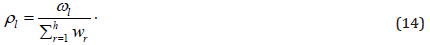
The kernel of prediction is a Takagi-Sugeno complex neurofuzzy system (TS-CNFS) used as the predictive model. When expanded, it contains six neural-network layers and is illustrated in Figure 1. These are the layers of input, complex fuzzy sets, activation, normalization and output, respectively. Each layer is formed by artificial neurons (termed nodes for simplicity). Nodes in each layer have specific functionality to be explained below.

Layer 1: Has M nodes in total corresponding to the inputs to the predictive model, respectively. The inputs are filtered (or selected) first by feature selection.

Layer 2: Contains nodes characterized by complex fuzzy sets. These nodes are termed as the complex fuzzyset nodes. Each input to the predictive model corresponds to a certain amount of nodes (that is, a group of nodes) in the layer. More specifically, the group size of nodes of one input can be different from that of another. Note that to form an if part (or termed a premise) with M conditions, each input provides a node from its group of nodes in Layer 2 to make the if part. Note that an if part is regarded as a node in Layer 3. 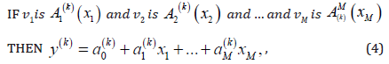Each of the M conditions of an if part can be expressed by a simple proposition with the form “𝑣 is 𝐴,” where 𝑣 is a linguistic variable and 𝐴 is a linguistic value. As a result, an if part is expressed by a complex proposition in the form of statement “𝑣₁ is 𝐴₁ and … and 𝑣_𝑀 is 𝐴_𝑀 ”, where each of the M inputs is regarded as a linguistic variable with its value. For the ith linguistic variable 𝑣_𝑖 , there is a term set symbolized as 𝑇_𝑖, whose size (cardinality) is denoted as , containing a group of linguistic values The term set 𝑇_𝑖 is expressed as follows.

where 𝐴_𝑖,𝑗 is the jth linguistic value of the ith variable. Accordingly, layer 2 has M groups of nodes corresponding to M term sets of linguistic values, respectively. Consequently, there are nodes in layer 2. For the linguistic value 𝐴_𝑖,𝑗, a node is characterized mathematically using a complex fuzzy set. A complex fuzzy set is an advanced fuzzy set whose complex-valued membership function 𝜇 is given as μ (x) = r (x)⋅exp( jω (x)), where 𝑟(𝑥) is the amplitude function with the restriction 0 ≤ r (x) ≤1;ω (x) is the phase function with the restriction ω (x)∈R; j² = −1; x is a generic numerical variable. This paper presents the following membership function design for complex fuzzy sets.

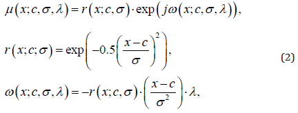
where {𝑐, 𝜎, 𝜆} are the parameters of {center, spread, phase factor} of a complex fuzzy set. The class of complex fuzzy sets defined by equation (2) is termed as Gaussian complex fuzzy sets [17], for their membership functions share the same basis using a Gaussian function and its first derivative with respect to 𝑥. In general, μ (x;c;σ ,λ ) is a complex-valued function, which can be expressed as μ (x;c;σ ;λ ) = Re((x;c;σ ;λ )) + j Im(μ (x;c;σ ;λ )) , where Re(⋅) and Im(⋅) are the real and imaginary parts, respectively. For the complex fuzzy set of 𝐴_𝑖,𝑗 , the complex-valued membership function is denoted as 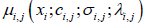⋅ The parameters are termed as the set of complex fuzzy set parameters, which are to be optimized by the method of MCACO. For the prediction of multiple targets, the output of the node for 𝐴_𝑖,𝑗 in Layer 2 is arranged to be a vector, denoted as , whose components are derived from the membership information of ⋅ (denoted as μ_𝑖,𝑗 for simplicity), for example real and imaginary parts as well as the μ_𝑖,𝑗 itself, given below.

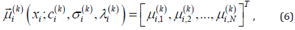
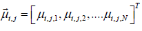, where N is the vector size. (3)

Layer 3: Contains K nodes, each of which represents an if part with M conditions. An if part and a then part (or termed a consequence) can make an if-then rule. The nodes of the layer represent K if parts in total, and therefore if-then rules to make. The type of Takagi-Sugeno (TS) if-then rules is adopted in the paper. The kth TS rule (for k=1, 2, …, K) can be expressed as follows.

where 𝑣_𝑖 is the ith input linguistic variable whose base (numerical) variable is denoted as is the linguistic value of 𝑣_𝑖 in the if part of the kth rule and is defined using a complex fuzzy set, whose complexvalued membership function is a function of 𝑥_𝑖 and is denoted as 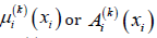for convenience. Note that the linguistic value is a linguistic value from the term set 𝑇_𝑖 given in equation (1). For the then part of equation (4), it is a TS linear function of the input base variables {𝑥_𝑖, 𝑖 = 1,2, … , 𝑀}, whose parameters are called the consequent parameters of the kth rule, which are to be optimized by the method of RLSE. For the complex fuzzy set of , using equation (2), the membership function is denoted as 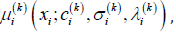given below.

are the parameters of the complex fuzzy set of . For multitarget prediction, a vector based on given in (5) is arranged as follows.

where denotes the qth component of the vector . Note that 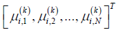can be arranged using the information by , for example 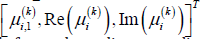(for N=3 in the case) or other possible forms, depending on applications. We apply the fuzzy-and operation, using the “product” implementation, to aggregate the propositions of the if part of the kth rule in [4].

The output of the kth node of layer 3, which is the activation level vector of the kth if part (or regarded as the rule’s firing strength vector for multiple outputs), is given in a vector form below.

where the qth component of is given as 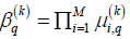(for q=1,2,…,N). Note that the vector is a complex vector due to part of its components are complex.

Layer 4: Performs the normalization of . There are K nodes performing the normalization in this layer, where each node receives all from layer 3. The output of the kth node is in a vector form given below.

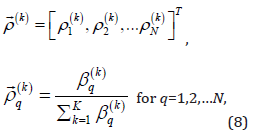
where the qth component of . The is a complex vector for all the components are complex after the normalization of .

Layer 5: Performs the TS then parts. There are K nodes for such a purpose in this layer. The output of the kth node is in a vector form given below.

where is called the augmented input vector and is the consequent parameter vector of the TS then part of the kth rule. With the method of RLSE, the set of parameters of in equation (9) are to be optimized.

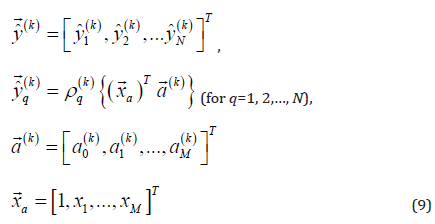
Layer 6: Summarizes the outputs of layer 5 to obtain the vector of multiple model outputs, given below.

where is the qth component of the model output vector . As shown in equation (10), the qth model output component is complex due to and thus can be expressed as 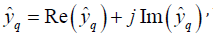which can be applied to dual-target applications. Note that the model output vector can theoretically be applied to applications with 2N real-valued targets.

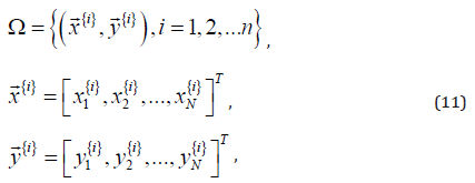
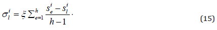
The flowchart of the prediction system is shown in Figure 2. From left to right, there are three sub-flowcharts: the method MCACO, the T-S complex neuro-fuzzy system and the method RLSE. The whole procedure starts at the first step of the MCACO and ends by the last step of the MCACO. Multiple ant colonies of MCACO in a cooperative way search for the solution of complex fuzzy set parameters in layer 2 of TS-CNFS. The RLSE method is responsible for the solution of TS consequent parameters in layer 5 of TS-CNFS. And, the MCACO and RLSE methods work together concordantly as one method, so to be named the MCACO-RLSE method. Each ant of the multiple ant colonies is evaluated by its performance in the machine learning process. A performance (or termed cost) criterion which is used to evaluate every ant is an error index. The training data set (Ω) for the machine learning of the proposed predictive model is expressed below [17-48].

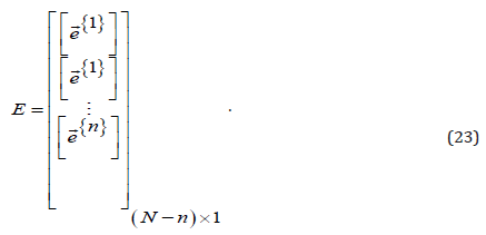
where {𝑖} indicates the ith pair of is the ith data pair of (input, target); is the input vector of the ith pair and is the target vector; n is the size of Ω. The performance of each ant in the MCACO is evaluated by the mean square error (MSE), the so-called cost function, defined below.

where is the qth component error (q=1,2,…,N) between the target vector and the model output vector given in equation [10] when the ith training data pair is presented to the predictive model; indicates the complex conjugate of . The MCACO-RLSE method is specified in detail in the following.

Machine Learning Method: MCACO-RLSE

Multi-swarm continuous ant colony optimization

In the paper, the problem under discussion is to minimize an objective function f(X) without constraints. The variable X is a parameter set used in layer 2 of the prediction system, i.e. every parameter set {𝑚, σ, λ} of all used complex Gaussian membership functions. Function f(X) evaluates the root-mean-squared error between the predicted and the expected when the current variable X is used. The method MCACO is proposed based on the method continuous ant colony optimization (CACO) [26]. However, the fore uses multiple ant colonies and an ant in different colony represents different part of the whole parameter set X. Thus, a whole parameter set is divided into several small sets so that every colony searches only in a small solution space. This is more effective than searching a whole large solution space.

Mechanism of generating new ants: Different colony searches for different part of the whole parameter set. Thus, only ants of the same colony are used to generate their own new ants. Initially, all ant colonies are randomly generated where every ant in different colony represents a different part of parameter vector X. When all ants in a colony have been evaluated, a key ant is randomly selected to generate new ants. The key ant decides how a Gaussian function of weighting probability is distributed. Based on these Gaussian distributions, new ants are therefore generated by contiguously recombining the parameters selected one by one from current ant colony. The mechanism of selecting key ant is like the way of playing roulette wheel. In current ant colony, all ants are ordered according to their objective function values f(X) from small to large. In the ant sequence, the lth ant’s weighting can be obtained as below.

There are total h ants in the colony and q is a learning parameter between 0 and 1. The larger the weighting 𝜔_𝑙 is the better the solution that the lth ant represents is. The selection probability is therefore calculated based on equation (8).

Assume the lth ant is selected as the key ant. Thus, its ith parameter is used as the averaged value and the corresponding standard deviation is shown as below.

The parameter 𝜉 is an evaporation rate. Of the ith parameter, the Gaussian function of weighting probability 𝐺𝑖(𝑥) is distributed as follows.

In words, different parameters have different distributions of weighting probability. A new ant is therefore created by recombining the parameters selected one by one.

Three strategies of ant evolution: Ants in different colonies represent different parts of the whole parameter set. Three strategies are therefore introduced to evaluate ants. By these strategies, all ant colonies are iteratively renewed to improve machine learning.

a. Evaluation strategy: An ant can be evaluated only if it becomes a whole parameter set. By the evaluation strategy, every ant in some colony is evaluated when combined with every the best ant in the other colonies. Initially, a randomly selected ant is used when the colony haven’t been evaluated yet. The strategy helps effective machine learning.

b. Elimination strategy: The elimination strategy is to totally renew the worst colony in where the best ant is the worst among all. Such colony will take time in machine learning. However, it may contain potential ants. The way to renew the whole worst colony is to generate sufficient new ants using the current ants and then replace all the latter.

c. Inheritance strategy: Ants in colonies perform well, i.e. with small root mean-squared error, because of containing good parameters. The inheritance strategy tries to keep these good parameters for next machine learning. Therefore, in order to renew such a colony, a specific number of top ants are kept while the rest are replaced by newly generated ants.

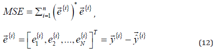
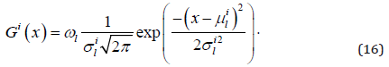
The flowchart of method MCACO is shown in Figure 3. The first step is to specify the parameters of MCACO, i.e. the number of total iterations, the number of total ant colonies, the number of top ants to be kept, the number of top best ants in every colony to be collected into the generation pool etc. Then, randomly generate ants as the first generation of all colonies. The evaluation to an ant is a root mean-squared error between the expected and the predicted when the ant combined with every the best of rest colonies is applied to the prediction system. When all ants of all colonies have been evaluated, all current colonies are then renewed and replaced by the three strategies until the number of total iterations has been reached.

Recursive least squares estimation (RLSE) for multiple targets

The RLSE method devotes to estimate all consequent parameters of the predictive model for multiple targets. Based on the method of least squares estimation, the RLSE method for the problem of linear regression optimization is efficient. A general least squares estimation problem is specified by a linearly parameterized expression given as follows.

where x is the input to model; y is the target; 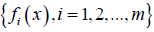are known functions of ; are the parameters to be estimated; 𝑒 is the error. With the training data set (Ω), we have the equation set given below.

In matrix notation, (18) can be rewritten as follows.

Where,

The consequent parameters of the predictive model can be arranged to be a vector that is regarded as the vector θ . For the recursive process of RLSE, a training data pair of Ω is presented at each recursive iteration. The next iteration follows based on the result of the previous one. The process goes on until all data pairs of Ω have been presented to finish one recursive epoch. The optimal estimate of θ , in terms of the minimum sense of , can be obtained using the training data pairs of Ω recursively by the following RLSE equations.

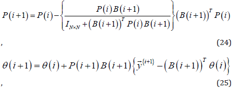
for 𝑖 = 0,1, … , (𝑛 − 1), where the index 𝑖 indicates the ith recursive iteration; 𝑛 is the number of training data pairs of Ω; N is the size of is the target vector of the (𝑖 + 1)th data pair; 𝐏(𝑖) is a m-bym projection matrix at the ith recursive iteration; I_N×N denotes the N-by-N identity matrix; initially 𝐏(0) = α I_mxm; α is a very large positive value and I_m×m is the m-by-m identity matrix. The transpose of (𝐁(𝑖 + 1)) in the RLSE equations is the ith row block of 𝐀, that is,

Note that the RLSE given above is to deal with multiple targets simultaneously and recursively.

For the implementation of RLSE on the predictive model with the training data set Ω in the learning

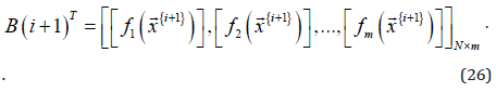
T process, the (𝐁(𝑖 + 1)) is given below.

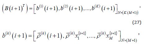
where the index k indicates the kth if part (𝑘 = 1,2, … , 𝐾 ) and the index (𝑖 + 1 ) indicates the (𝑖 + 1 )th recursive iteration; is specified in equation [8]; is the jth component (j=1,2,…,M)) of the input vector given in (11); {𝑀, 𝑁, 𝐾} are the numbers of inputs, outputs and if-then rules of the predictive model,

T respectively. Note that when equation (26) compares with (27) for the dimension of (𝐁(𝑖 + 1)) , the equation 𝑚 = K ⋅(M +1) holds. And, the vector of consequent parameters of the predictive model is given as follows.

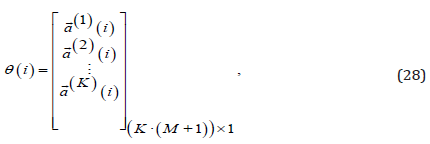
where is the consequent parameter vector of the kth TS then part (k=1,2,…,K) at the ith recursive iteration of RLSE. The optimal estimate for θ is θ (n), where 𝑛 denotes the final recursive iteration when one RLSE epoch is done. The procedure of the proposed MCACO-RLSE is summarized as follows.

Step 1. Initialize the setting of MCACO-RLSE. Start the MCACO.

Step 2. Calculate membership degree vectors of complex fuzzy sets in layer 2. Obtain the firing strength vectors in layer 3 and do the normalization in layer 4 for these vectors of the predictive complex neuro-fuzzy model.

Step 3. Update the consequent parameters in layer 5 of the model by the RLSE.

Step 4. Calculate forecast vector by the model and obtain error vector for each training data pair until all data pairs have been presented. Get the cost of ant in MSE.

Step 5. Calculate the cost of each ant of MCACO by repeating Steps 2 to 4 until all ants are done. Obtain the best ant position so far for each of the multiple swarms. Combine the positions of the best ants of the ant swarms together to get the solution so far to update the parameters of complex fuzzy sets in layer 2 of the predictive model.

Step 6. Check for any of stopping conditions to stop. Otherwise go back to Step 2 and continue the procedure.

Feature Selection Crossing Multiple Targets

Feature selection is a method of selecting a compact set of important features out from candidate features. These selected features are used as the inputs to the prediction system with multiple targets. In the paper, the inputs and outputs of the prediction system are difference values of real observations. For multiple target prediction, a two-stage feature selection is proposed, where useful features for each single target are determined explicitly in the first stage and, based on the determined in stage 1, those features significant to all targets are selected in the second stage. Suppose that there are a set of candidate features to be selected in the procedure of feature selection in which multiple targets are considered. Let the candidate features be placed in a pool called the candidate feature pool denoted as C_p, given below.

where 𝑋𝑘 is the kth candidate feature of denotes the size of 𝐶𝑝. The multiple targets considered in the feature selection procedure is given as follows.

where 𝑌_𝑖 is the ith target in the set T whose size is denoted as . All the candidate features of C_p and the targets of T are regarded as random variables.

Stage 1 of Feature Selection

Assume there is a target denoted as 𝑌 from the target set T. Let 𝐻(𝑌) denote the entropy of target 𝑌, where 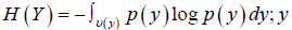s a generic event of Y; U(𝑦 ) is the universal event set for 𝑦 ;

𝑝(𝑦) is the probability density distribution of 𝑦 . From the candidate feature pool C_p , a feature 𝑋 is considered. Let the feature X be separated into two parts 𝑋⁺ and 𝑋⁻ , where 𝑋⁺ and 𝑋⁻ denote the positive and negative parts of X, respectively. That is, the values of 𝑋⁺ are positive and those of 𝑋⁻ are non-positive. Let 𝐻_𝑋+(𝑌) denote the entropy of target 𝑌 conditioned by feature 𝑋⁺ . According to the Shannon’s information theory [11], the mutual information between 𝑌 and 𝑋⁺ is given as 𝐼(𝑋⁺, 𝑌) = 𝐻(𝑌) − 𝐻_𝑋+(𝑌) . Now another idea of information called the influence information is defined for the influence made by feature 𝑋 to target 𝑌. Such influence information is denoted as I_x→y given below.

where 𝑝(𝑥)is the probability density distribution of x, a generic event of feature X. Note that the distributions of 𝑝(𝑥) and 𝑝(𝑦) can be estimated by density estimation [44]. Note that the integration indicates the probability of 𝐼(𝑋⁺, 𝑌) and the probability of 𝐼(𝑋⁻, 𝑌). In contrast to the symmetry of Shannon’s mutual information, the influence information given in (31) is asymmetric, that is, I_x→y≠I_y→x.

The first stage procedure of feature selection is given below.

Step 1. Prepare each target of T a pool to contain features to be selected from Cp. For target 𝑌𝑖 of T, the pool is termed the selected features pool for it, denoted as S𝑌𝑖, for i =1,2,..., T ⋅ Initially S𝑌𝑖 is empty.

Step 2. Let C_𝑌𝑖 be the pool containing all the candidate features for a target 𝑌_𝑖, that is,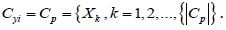

Step 3. Calculate the mutual information of 𝑌_𝑖, to which compute influence information of each candidate feature of C_𝑌𝑖 . For each candidate feature, calculate selection gain. The selection gain of 𝑋_𝑘 of C_𝑌𝑖 making contribution to target 𝑌_𝑖 is defined as follows.

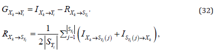
for where G_{Xk → Y=Yi} is the selection gain when selecting feature 𝑋_𝑘 into the pool S𝑌𝑖 for target 𝑌_𝑖; R_{Xk → Y =SYi} is an averaged redundant information made by feature 𝑋_𝑘 to all selected features already in the pool S_𝑌𝑖 so far; S_𝑌𝑖(𝑗) indicates the jth feature already in the pool S_𝑌𝑖 so far; is the size of S𝑌𝑖 so far. Note that the selection gain indicates the measure of significance for a random variable making influence/ contribution to another.

Step 4. Check for the candidate feature whose selection gain is the largest over all other ones in C_𝑌𝑖. If it is positive, update the pools C_𝑌𝑖 and S_𝑌𝑖, as follows.

where 𝑋_𝑚 indicates the candidate feature with the positive max selection gain over all other ones in C_𝑌𝑖 so far; C_𝑌𝑖 ⊝ 𝑋_𝑚 means the operation of excluding 𝑋_𝑚 from C_𝑌𝑖 and S_yi ⊕ X_m means the operation of including 𝑋_𝑚 into S_𝑌𝑖. Otherwise, go to step 6.

Step 5. If go to step 6. Otherwise, go back to step 3.

Step 6. If update 𝑖 = 𝑖 + 1 to get next target and go back to step 2. Otherwise, stop the procedure and output all the selected feature pools and S_yi (j) is the jth selected feature in S_𝑌𝑖 for target 𝑌_𝑖.

Stage 2 of Feature Selection

For each target in the target set T, the result has been done with the first stage of feature selection, as shown in , based on which the second stage of feature selection goes on for further consideration of multiple targets. For , the contribution by each of all the selected features to all targets will be inspected separately. Thus, the features that are globally important to all targets can be decided. The feature selection procedure of stage 2 is given below.

Step 1. Identify exclusively all the features that are in the pools .

These features are placed into a set denoted as Ω = where φ_k is the 𝑘th feature of Ω.

Step 2. Compute coverage rate of each feature in Ω to all the targets .

Compute the count of φ_k in the pools denoted as And, compute the coverage rate of φ_k to all the targets, denoted as ω(φ_k), given below.

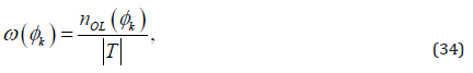
for denotes the size of Ω. Compute

Step 3. Compute contribution index of each feature in Ω to all the targets.

Compute the contribution index by φ_k to all the targets, denoted as ρ(φ_k), given below.

Step 4. Test the features in Ω for the following condition.

If where is termed the condition threshold; 𝑛_tmp records the number of feature variables in Ω fulfilling the condition above. Note that the condition threshold ρth can also be set in other ways.

Step 5. Decide the finally selected features.

Set lower and upper limits for finalizing the number of feature variables. These features are placed finally in the so-called final pool (FP). The lower and upper limits are denoted as 𝑛_L and 𝑛_U, respectively. The number of features in F_P is denoted as 𝑛_F or . Note that 𝑛L and 𝑛U are set depending on application. The 𝑛_tmp is obtained in step 4.If n_tmp < n_L , then 𝑛_F = 𝑛_L, elseif n_L ≤ n_tmp ≤ 𝑛_U, then 𝑛_F = 𝑛_tmp, else 𝑛_F = 𝑛_U, end. After ranking , select top 𝑛F corresponding features {𝑓_𝑖, 𝑖 = 1,2, … , 𝑛_F} and place them into the final pool F_P, given as follows.

where 𝑓_𝑖 is the 𝑖th feature of F_P contributing to all the targets given in the set T.

Results and Discussion

Real world stock-market data are utilized to test the proposed approach. In experiment 1, the proposed system is to make dual outputs at the same time to predict the Taiwan capitalization weighted stock index (TAIEX) and the SSE composite index (SSECI) posted by Shanghai stock exchange. Experiment 2 is to make triple outputs simultaneously for prediction of three stock indexes, i.e. SSECI, the Standard & Poor’s 500 (S&P 500) and Dow Jones industrial average (Dow Jones). Table 1 shows the model setting of our prediction system. The number of model outputs depends on how many targets to be predicted. For experiment 1, two real-valued targets (TAIEX and SSECI) are placed into the real and imaginary parts of a complex-valued target, respectively, to which the TS-CNFS needs only one complex-valued output to make prediction. For experiment 2 with three real-valued targets, the TSCNFS model may need two complex-valued outputs, corresponding to two complex-valued targets. The first two of the three realvalued targets (SSECI, S&P 500 and Dow Jones) are placed into one complex-valued target and the third one is placed into the real part of the other complex-valued target whose imaginary part is placed with zero. Table 2 shows the parameters of approach MCACO-RLSE used for all the experiments.

Experiment 1: The prediction of TAIEX and SSECI is carried out by the proposed approach. All gathered data of close prices cover the whole year 2006. The data of the first ten months are used for training and those of the last two months are used to test and evaluate the performance of the prediction system. In the case, 15 features for each target are gathered so that there are total 30 candidate features. By the proposed feature selection, three features are selected as inputs to the prediction system. The first feature is selected from the features of TAIEX and the rest two from SSECI. Thus, the prediction system has total 27 TakagiSugeno if-then rules with one complex output. Table 3 shows performance comparison in terms of root mean square error by the proposed approach (in test phase) to nine compared methods in literature. The dual predictions during testing phase are outstanding. As shown in table 3, by our prediction system, both the predictions of TAIEX and SSECI have improved with 6% and 8% when compared with those obtained by Zhang et al. [36]. The performance by the proposed approach performing prediction of dual targets is superior to the compared methods in literature, even each of the compared is for prediction of one target only. The proposed prediction system demonstrates outstanding dual-predictions by using one complex valued model output for two real-valued targets. Moreover, as shown in this case the proposed MCACORLSE method has shown effective ability of machine learning through the empirical result. Furthermore, such successful performance only uses three inputs obtained by the proposed feature selection.

Experiment 2. The prediction of SSECI, S&P500 and Dow Jones is carried out by the proposed approach. All data are gathered from year 2006 to year 2012, where most of them are for training and the rest for testing. By the feature selection, thirty candidate features for each target are gathered, and there are total ninety candidate features., Three features eventually are selected from the ninety candidate features. The predictive model with two complex outputs for prediction of SSECI, S&P500 and Dow Jones. Performance comparison by the proposed model after training to the compared methods in literature is given in Table 4, showing the performance of the proposed model is superior to the compared methods, in terms of in terms of root mean square error.

Conclusion

The prediction system using complex fuzzy sets has been successfully developed and tested. The hybrid machine learning MCACO-RLSE method associated with the two-stage feature selection for the proposed model has achieved multi-target prediction in the experimentation. Through performance comparison with other methods in literature, as shown in Tables 3 & 4, the proposed approach has shown excellent performance.

Acknowledgement

This work was supported by the research projects MOST 105-2221-E-008-091 and MOST 104-2221-E008-116, Ministry of Science and Technology, TAIWAN.

References

1. Engle RF (1982) Autoregressive Conditional Heteroscedasticity with Estimates of the Variance of United Kingdom Inflation Econometrica 50(4): 987-1007.
2. Bollerslev T (1986) Generalized Autoregressive Conditional Heteroscedasticity Journal of Econometrics 31: 307-327.
3. Widrow B, Hoff ME (1960) Adaptive Switching circuits Proc. IRE WESCON Convention Record. USA.
4. Kimoto T, Asakawa K, Yoda M, Takeoka M (1990) Stock market prediction system with modular neural networks Proc. International Joint Conference. USA.
5. Kim K, Han I (2000) Genetic algorithms approach to feature discretization in artificial neural networks for prediction of stock index Expert System with Applications 19: 125–132.
6. Roh TH (2007) Forecasting the volatility of stock price index Expert Systems with Applications 33: 916–922.
7. Zadeh LA (1965) “Fuzzy sets”, Information and Control 8(3): 338-353.
8. Ramot D, Milo R, Friedman M, Kandel A (2002) Complex fuzzy sets IEEE Transactions on Fuzzy Systems 10(2):171-186.
9. Takagi T, Sugeno M (1985) Fuzzy identification of systems and its applications to modeling and control IEEE Trans. Syst. Man Cybern 15: 116–132.
10. C Li, Chiang T (2013) Complex Neuro fuzzy ARIMA Forecasting - A New Approach Using Complex Fuzzy Sets IEEE Transactions on Fuzzy Systems 21(3): 567-584.
11. Colorni A, Dorigo M, Maniezzo V (1991) Distributed optimization by ant colonies Proc. of the 1st European Conference on Artificial Life. France.
12. Socha K, Dorigo M (2008) Ant colony optimization for continuous domains European Journal of Operational Research 185(3): 1155–1173.
13. Shannon CE, Weaver W (1949) The Mathematical Theory of Communication Univ. of Illinois Press. USA.
14. E Parzen (1962) On estimation of a probability density function and mode Annals of Math. Statistics (vol. 33): 1065-1076.
15. Kwak N, Choi CH (2002) Input feature selection by mutual information based on Parzen window IEEE Transactions on Pattern Analysis and Machine Intelligence 24(12): 1667-1671.
16. Peng H, Long F, Ding C (2005) Feature selection based on mutual information: Criteria of maxdependency max-relevance and minredundancy IEEE Transactions on Pattern Analysis and Machine Intelligence 27(8): 1226–1238.
17. Laney D (2001) 3D Data Management: Controlling Data Volume, Velocity and Variety META Group Research Note.
18. Juang C, Jeng T, Chang Y (2015) An Interpretable Fuzzy System Learned Through Online Rule Generation and Multiobjective ACO With a Mobile Robot Control Application. IEEE Transactions on Cybernetics. 46(12): 2706-2718.
19. Sadaei HJ, Enayatifar R, Lee MH, Mahmud M (2016) A hybrid model based on differential fuzzy logic relationships and imperialist competitive algorithm for stock price forecasting Applied Soft Computing 40: 132- 149.
20. Kennedy J, Eberhart RC (1995) Particle swarm optimization in Proc. IEEE International Conference on Neural Networks (vol. 4). Australia.
21. Eberhart RC, Kennedy J (1995) A new optimizer using particle swarm theory in Proc. IEEE International Symposium on Micro Machine and Human Science. Japan.
22. Powell WB (2011) Approximate Dynamic Programming: Solving the Curses of Dimensionality John Wiley & Sons, Inc. Hoboken New Jersey. USA.
23. Kira K, Rendell L (1992) A practical approach to feature selection Proc. of the Ninth International Conference on Machine Learning. Scotland.
24. H Yu J Oh, Han WS (2009) Efficient feature weighting methods for ranking Proc. of the 18th ACM Conference on Information and Knowledge Management, China.
25. Clausius R (1854) Ueber eine vera nderte Form des zweiten Hauptsatzes der mechanischen Wa rmetheorie Annalen der Physik und Chemie 93(12): 481–506.
26. Cantor G (1874) Ueber eine Eigenschaft des Inbegriffs aller reellen algebraischen Zahlen Journal fu r die reine und angewandte Mathematik 77: 258-262.
27. Russell B (1923) Vagueness Australasian Journal of Philosophy 1(2): 84- 92.
28. Max B (1937) Vagueness: An exercise in logical analysis Philosophy of Science 4:427–455.
29. McCulloch WS, Pitts W (1943) A logical calculus of the ideas immanent in nervous activity The bulletin of mathematical biophysics 5(4): 115- 133.
30. Widrow B, Hoff ME (1960) Adaptive Switching circuits Proc. IRE WESCON Convention Record. USA.
31. Rumelhart DE, McClelland JL (1986) Parallel distributed processing: explorations in the microstructure of cognition vol. 1: foundations. MIT Press Cambridge MA, USA.
32. Socha K, Dorigo M (2008) Ant colony optimization for continuous domains European Journal of Operational Research 185(3): 1155–1173.
33. Huarng K, Yu HK (2005) A Type 2 fuzzy time series model for stock index forecasting Physical A: Statistical Mechanics and its Applications 35: 445-462.
34. Cheng CH, Cheng GW, Wang JW(2008) Multi-attribute fuzzy time series method based on fuzzy clustering Expert Systems with Applications 34(2): 1235-1242.
35. Chen SM (2002) Forecasting Enrollments Based On High-order Fuzzy Time Series Cybernetics and Systems 33(1): 1-16.
36. Lee LW, Wang LH, Chen SM, Leu YH (2006) Handling forecasting problems based on twofactors high-order fuzzy time series IEEE Transactions on Fuzzy Systems 14(3): 468-477.
37. Egrioglu E, Aladag CH, Yoclu U, Uslu VR, Erillli NA (2011) Fuzzy time series forecasting method based on Gustafson–Kessel fuzzy clustering Expert Systems with Applications 38(8): 10355-10357.
38. Wang L, Liu X, Pedrycz W (2013) Effective intervals determined by information granules to improve forecasting in fuzzy time series Expert Systems with Applications 40(14): 5673-5679.
39. Bas E, Yoclu U, Egrioglu E, Aladag CH (2015) A Fuzzy Time Series Forecasting Method Based on Operation of Union and Feed Forward Artificial Neural Network American Journal of Intelligent Systems 5(3): 81-91.
40. Yoclu OC, Yoclu U, Egrioglu E, Aladag CH (2016) High order fuzzy time series forecasting method based on an intersection operation Applied Mathematical Modeling 40(19-20): 8750-8765.
41. Zhang W, Zhang S, Zhang S, Yu D, Huand NN (2017) A multi-factor and high-order stock forecast model based on Type-2 FTS using cuckoo search and self-adaptive harmony search Neurocomputing 240: 13-24.
42. Hassan MR, Nath B (2005) Stock Market Forecasting Using Hidden Markov Model: A New Approach Proc. Fifth International Conference on Intelligent Systems Design and Applications. Poland.
43. Hsieh TJ, Hsiao HF, Yeh WC (2011) Forecasting stock markets using wavelet transforms and recurrent neural networks: An integrated system based on artificial bee colony algorithm Applied Soft Computing 11(2): 2510-2525.
44. Wang J, Wang J (2015) Forecasting stock market indexes using principle component analysis and stochastic time effective neural networks Neurocomputing 156: 68-78.
45. Huarng KH, Yu THK, Hsu YW (2007) A Multivariate Heuristic Model for Fuzzy Time-Series Forecasting IEEE Transactions on Systems Man and Cybernetics Part B 37(4): 836-846.
46. Chen SM, Tanuwijaya K (2011) Multivariate fuzzy forecasting based on fuzzy time series and automatic clustering techniques Expert Systems with Applications 38(8): 10594-10605.
47. Chen SM (1996) Forecasting enrollments based on fuzzy time series Fuzzy Sets and Systems 81(3): 311-319.
48. THK Yu, Huarng KH (2008) A bivariate fuzzy time series model to forecast the TAIEX Expert Systems with Applications 34(4): 2945-2952.