Optimization of Waste Discharge Points in Natural Streams Volume 2 - Issue 5

Ezeilo FE¹ and Agunwamba JC²*

• ¹Department of Civil Engineering, Rivers State University of Technology, Nigeria
• ²Department of Civil Engineering, University of Nigeria, Nigeria

Received: August 09, 2018;   Published: August 28, 2018

Corresponding author: Agunwamba JC, Department of Civil Engineering, University of Nigeria, Nsukka, Enugu State, Nigeria

DOI: 10.32474/TCEIA.2018.02.000148

Abstract PDF

---

Abstract

This paper reports on a study carried out to optimize the locations of multiple discharge points in a receiving stream, Amadi creek, so as to minimize the impact of oxygen demanding resources (BOD) on water quality. The study evaluated the water quality changes as a result of the increasing human and industrial activities around the creek. Water quality standards require the maintenance of dissolved oxygen (DO) concentration of 5mg/l or more at any time in streams. However practical analysis of the water samples from Amadi creek reveal a DO level as low as 2.3mg/l. The DO deficit was computed from data generated by sampling DO concentrations along the creek from various points of waste discharge downstream while the BOD of the stream was determined by monitoring BOD of samples obtained along the creek. The study also identified and quantified the amount of effluent entering the creek from various point sources. The DO deficit equations are solved by the methods of simple calculus (classical optimization), which simplifies the mathematical solution of the model equations by avoiding difficult to evaluate integrals Two scenarios were identified and used to investigate the effect of BOD on the DO level in the stream, using mathematical simulation techniques. Simulation results show that to ensure minimum impact of BOD on water quality waste discharge locations should be placed at the optimal locations of 10015.382m and 6992.282m upstream and downstream waste discharge points respectively, at an optimum DO deficit of 4.135mg/l for case 1.

For case2, the waste discharge locations are to be placed at optimal locations 40995.43m, 30665.17m, 41233.69m upstream and downstream waste discharge points respectively at an optimum DO deficit of 4.567mg/l. This means that if a new waste input is proposed for a stream its BOD input and its proposed location with respect to other inputs are important in order to determine the effect on the DO level in the stream Discharges from the second treatment plant would result in decreased dissolved oxygen level for a substantial distance downstream. This can have significant effects for streams and rivers with many influent waste streams over their course, as the dissolved oxygen (DO) will not have a chance to recover between each influent stream, resulting in significantly depressed oxygen levels .The dissolved oxygen (DO) deficit becomes zero at approximately the same distance downstream for both cases, though the two point source discharge case (case2) shows a higher short term DO deficit. This can cause problems if they DO concentration drops below the stipulated levels for the creek, leading to possible death of fish and other aquatic lives. It is therefore recommended that industrial establishments planning to site their treatment facilities along rivers or streams should be compelled to discharge their waste stream in compliance with the optimal locations with respect to any existing plant, so as to avoid undue dissolved oxygen (DO) depletion.

Keywords: Point Sources; Effluent; Discharge Point; Impact, Creek; Optimal Location; Sampling

Introduction

Modeling the impact of Biological Oxygen Demand (BOD) on water quality is an important part of the permitting process for new resources Masters [1]; Agunwamba et al. [2]; Peavy et al. [3]. Many rivers and streams in Port-Harcourt metropolis, Nigeria as a whole and indeed all over the world have suffered from dissolved oxygen (DO) deficit, which is very crucial to survival of aquatic life. Stream models can help determine the maximum amount of additional BOD that will be allowed, which, in turn, affects facility siting decisions and the extent of on-site waste water treatment that will be required Agunwamba et al. [2]; Mcbride [4] ; Ezeilo et al. [5]; Dobbins [6] .The amount of dissolved oxygen (DO) in water is one of the most commonly used indicators of a rivers health ( Ezeilo et.al, 2012 ). As DO drops below 4 or 5 mg/l, the forms of life that can survive begin to be reduced. In the extreme case when hypoxic conditions (0<DO<5mg/l) exist, most higher forms of life are killed or driven off. Among the factors affecting the DO available in a stream are BOD, which account for the oxygen demanding wastes Brown [7]; Ezeilo et al. [8], Ezeilo et al. [9]. Photosynthesis also affect DO. Algae and other aquatic plants add DO during the daytime hours, while photosynthesis is occurring, but at night their continued respiration draws it down again. The net effect is a diurnal variation that can lead to elevated levels of DO in the late afternoon and depressed concentrations at night. For a lake or a slow-moving stream that is already overloaded with BOD and choked with algae, it is not unusual for respiration to cause offensive, anaerobic conditions late at night, even though the river seems fine during the day. Other factors which would affect DO availability in a stream include, accumulated sludge along the bottom, tributaries, which mix with those of the mainstream. etc. Water quality modeling in a river has developed from the pioneering effort of Streeter and Phelps [10], who proposed a mathematical model demonstrating how DO in the Ohio River decreased with downstream distance due to degradation of soluble organic BOD.

According to Yudianto et al. [11] the simplest manifestation of this equation is usually applied for a river reach characterized by plug flow system with constant hydrology and geometry under steady state condition, as occurred in Amadi creek. For a large river or estuary, considerable longitudinal dispersion influences the phenomenon of DO and BOD distribution and so the governing equations becomes a partial differential equation. However, the effect of dispersion on DO and BOD in small rivers, like Amadi Creek, used in this study, is negligible Li [12]. Water collected for sampling is discharged into Amadi creek without any treatment as point source. Therefore, specifically Amadi creek is modeled with single point source of BOD in this study. Much research has been done on the area of DO depletion in water bodies, providing information on critical deficit, critical distance, and minimum DO concentration, but none of these studies has attempted to optimize the waste discharge locations for minimum impact of oxygen demanding resources (BOD) on water quality. This would have enabled us to establish an optimum deficit and optimum discharge locations for minimum impact of oxygen demanding resources on water quality. Such a study has been undertaken in Amadi Creek. This research was therefore carried out to identify and quantify the amount of waste water effluent entering the creek and evaluate the impact of these oxygen demanding wastes on water quality. A novel approach that will help minimize stream pollution when there are many industries discharging waste water into a stream is presented. Also, the determination of points of maximum DO deficit in case of multiple discharges along a stream using classical optimization technique is discussed.

Brief Description of the Study Area

The Amadi Creek has the Bonny river as its major source. It flows from Okrika down to Mini-Ewa, Rumuobiakani through Woji, Oginigba, Okujagu communities and back to the Bonny river where it empties out into the Atlantic oc ean. Amadi creek is located in Obio-Akpor Local Government Area and is host to several industries and factories as well as the popular Port-Harcourt city abbatoir (Slaughter). A sketch of Amadi Creek showing point sources of pollution are shown in Figure 1.

Methodology

Data was generated by sampling DO concentrations along the creek aboard a boat from various waste discharge locations and monitoring the BOD of samples obtained along the creek. The water temperature and pH was also determined. Other parameters determined include creek depth, width, flow velocity and flow rates. The BOD and DO were determined following the procedures given in the standard methods ( Apha,1998). Samples were collected with winkler bottles at intervals downstream, sealed to exclude air bubbles and sent to the laboratory for analysis. The depth were measured by dropping a loaded tape to the bottom of the creek, while the width was measured by stretching a tape across the creek. Temperature was measured on site using a clinical thermometer, while velocity was determined with a current meter.

Theoretical Formulation

Case 1 – One Source of Waste Water Discharge (Figure 2)

The dissolved oxygen deficit along the reaches are:

where, Lo is ultimate BOD concentration upstream effluent discharge, Do initial Do concentration upstream effluent discharge

The concentrations just downstream are computed by a mass balance as;

where, Q 1, Q 2 are the stream and effluent discharges respectively. L 1, L 3 are BOD of stream upstream and downstream respectively, L 2 is BOD of Effluent discharge, D 1, 3, are the DO concentrations upstream and downstream respectively, D2, is the DO concentration of Effluent discharge. In the Streeter and Phelps derivation the differential for L is assumed as which integrates to;

Substituting equations (3) and (4) into eq (2), gives

Case 2 – Two Sources of Waste Water Discharge (Figure 3)

The dissolved oxygen deficit along the reach CD, gives;

where, Q4, Q5, are the stream and Effluent discharge respectively, L4, L6, are BOD upstream and downstream respectively, L 5 is BOD of Effluent discharge, D4, D5 are the DO concentrations of stream and Effluent respectively.

Substituting equations (7) and equation (8) into equation (6) gives:

Assumptions

a) The main assumption in the formulation of the equations is that the river reach is characterized by plug flow system with constant hydrology and geometry under steady state condition and is traveling at a constant speed (u).

b) It is also assumed that water temperature is constant throughout the stream. Mixing of different temperature streams is not accounted for.

c) It is assumed that there is a constant discharge of waste water into the creek and also that the waste water is discharged into Amadi creek without any treatment as point source. Therefore, specifically Amadi creek is modeled with single point source of BOD in this study.

Optimization Problem

The problem of searching for the optimal waste discharge locations, for minimum impact on water quality may be expressed (Figures 2 & 3) as;

Subject to, t₁>0, t₂>0

where, X₁ and ho are the optimal waste discharge locations

Equations (5) and (6) represents the mathematical models for the stated problem. This is an optimization (maximization) problem Nwaigwe [13]. The desired solution of the above problem involves the search for the optimal values of the waste discharge locations i.e. the optimal determination of the values of x1 and ho for each waste discharge point. This can be solved by the method of simple calculus as follows;

Case 1: The derivative of equation (5) when 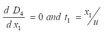is

Where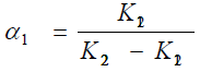

The derivative of e. q (5) when 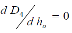is

Where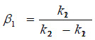

Hence the optimal locations X1 and ho at which the waste discharge locations will be placed for minimum impact on water quality are obtained by solving equations (11) and (12) as;

where X2 is the downstream location, and u is the average stream velocity, while t3 is the time of travel.

The derivative of e q (10) when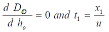

The derivative of eq when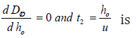

Hence the optimal locations X1, ho and X2 at which the waste discharge locations will be placed for minimum impact on water quality are obtained by solving equations (13), (14), (15) as;

x₁, ho and x₂ are the optimal waste discharge locations and Q₄ , Q₅, are the Stream and Effluent discharges respectively. L₅ and D₅ are the Effluent BOD and DO concentrations respectively. K₁₃, k₂₃ are the de oxygenation and re aeration rates respectively. As previously mentioned when eqn (1) and eqn (6) are assumed to be steady state, time (or distance) is the only independent variable. Equations (5) and (6) are the mathematical models for the problem of optimization of the waste discharge locations in rivers. These equations can be solved for the root t by a numerical root finding method in a software package such as MATHCAD or MATEMATICA. The value of t is then substituted into eqn (5) or eqn (6) to calculate the optimum DO deficit. An alternative procedure to finding the optimum DO deficit is to apply a series of times or velocities in eqn (5) and eqn (6) and record the value of the optimum DO deficit and the times or velocities to which it corresponds Nwaigwe [13]. Since the DO equations contain both DO deficit and t (which is a function of DO), the solution is thus arrived at by iteration using the Newton- Raphson method with the help of a developed VISUAL BASIC Programme.

Application of Models

The developed models were applied to the water quality data for Amadi Creek (Table 1). The input data for simulations of the two case studies are;

Case 1: Q1 = 0.139m³/s, Q2 = 0.5m³/s, Lo = 7.59 mg/l, Do = 4.1 mg/l

k11 = 0.1/day, k12 = 0.17/day, L2 = 20mg/l, k21 =0.17/day k22 = 0.23/day.

Case 2: Q5 = 0.65m³/s, L2 = 25 mg/l, D5 = 3.4 mg/l, k13 = 0.26/ day, k23 = 0.42/day

Substituting the above values in the above equations gives the optimal locations X1 and ho as10015.382m and 6992.282m respectively, at an optimum deficit of 4.135mg/l for case 1.Thus the model predicts that at an optimum deficit of 4.135mg/l the waste discharge locations would have to be placed at 10015.382m and 6992.282m upstream and downstream waste discharge locations respectively for minimum impact on water quality. For case 2, substituting these values in the above equations results in an optimum DO deficit of 4.567mg/l at optimal locations of 41233.43m, 40995.17m, 30665.69m upstream and downstream waste discharge locations respectively, to ensure minimum impact on water quality. The DO, BOD and temperature of the mixture effluent with creek water was obtained.

From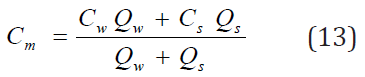

where Cm represents concentration of any parameter such as DO, BOD and water temperature at the point effluent mixes with creek water. The subscript denotes stream (or creek) and waste water respectively and Qs is the stream flow rate and Qw is the waste water flow rate. In order to convert BOD5 to ultimate BOD (Lo), using the first order decay rate, an extrapolation can be made according to Agunwamba et al. [2], as follows:

Effect of Flow conditions on Single Point Source Discharge

The result of the single point source case is presented in Figure 4. As expected the DO deficit curve rises to the point of optimum (maximum) deficit as the BOD is being degraded, and then start decreasing as the effect of the waste stream is felt approximately10000 meters downstream of the outfall. Here the stream becomes super-saturated due to the increased production of oxygen. This increased DO concentration may have been due to the activities of phytoplankton species living in the water (Ezeilo et.al 2012), and enhanced re aeration due to the optimum deficit of 4.135 mg/l. At this point, which corresponds to the point of maximum deficit, the stream undergoes a high level of re aeration. This is because DO deficit is the driving force for the replenishment of oxygen in polluted waters Sakalauskiene [14]. Thus, the greater the deficit, the greater the transfer of oxygen into the water Agunwamba [2]. After the point of maximum deficit, and high re aeration, the stream once again experiences a fall in the deficit as we move downstream, due to lesser concentration of the BOD, leading to improved DO concentrations, and so the DO equilibrates at a much higher concentration than in the two-point case. However, if there are other point sources downstream from the sewage treatment plant, the combined effect could cause significant depression of the stream DO concentration.

Effect of Flow Conditions on Two Sequential Point Source Discharge

The result of the two-point source discharge is presented graphically in Figure 5. They show the combined effect of a second sewage treatment plant some distance downstream. This second outfall is located in the region affected by the first out fall. The result shows a lowered DO deficit curve, shifting appreciably by the remaining DO deficit from the first outfall. This may have been due to increase in stream flow from the addition of the first out flow Ezeilo et al. [3]. This is also seen in the small change in the slope curve at the point of discharge. The second effluent stream results in a lowered DO concentration further downstream than for the single point case .This drop in the DO concentration could cause problems adjacent to the outfall if they DO concentration fall below the minimum standards set for the stream as observed by Brown [5] Due to increased effluent waste stream, very little oxygen is retained in the stream, resulting in a depressed DO deficit curve .Additionally, due to increased velocity, the travel time has significantly decreased and the resultant effect is a depressed DO concentration farther downstream than for the single point source case.

Conclusions and Recommendations

The dissolved oxygen (DO) deficit is dependent on the distance between multiple waste stream inputs (waste discharge points). This means that if a new waste input ( a new sewage treatment plant for example) is proposed for a stream or creek, both its BOD input and the proposed location with respect to other inputs are important in order to determine the effects on the dissolved oxygen (DO) level in the stream Discharges from the second treatment plant would result in decreased dissolved oxygen level for a substantial distance downstream. This can have significant effects for streams and rivers with many influent waste streams over their course, as the dissolved oxygen (DO) will not have a chance to recover between each influent stream, resulting in significantly depressed oxygen levels .The dissolved oxygen (DO) deficit becomes zero at approximately the same distance downstream for both cases, though the two point source discharge case (case2) shows a higher short term DO deficit. This can cause problems if they DO concentration drops below the stipulated levels for the creek, leading to possible death of fish and other aquatic lives. It is recommended that industrial establishments planning to site their treatment facilities along rivers or streams should be compelled to discharge their waste stream in compliance with the optimal locations with respect to any existing plant, so as to avoid undue dissolved oxygen (DO) depletion.

References

1. Masters GM (2007) Introduction to Environmental Engineering and Science. (2_nd edn) Pearson Education inc. USA pp. 259.
2. Agunwamba JC, Maduka CN, Ofosaren AM (2006) Analysis of Pollution Status of Amadi Creek and its Management. J of Water Supply: Res and Tech AQUA 55(6): 427-435.
3. Peavy HS, Rowe DR, Tchobanoglous G (1985) Environmental Engineering. International Edition. McGraw-Hill Book Company NY, USA pp. 85.
4. Mcbride GB (1982) Nomographs for rapid solutions for the Streeter- Phelps equations. J Wat Poll Control Feder 54(4): 378-384.
5. Ezeilo FE, Agunwamba JC ( 2014a) Effects of some functional parameters on DO deficit in a Natural Stream. Health, Safety and Environment Journal 2(3): 78-87.
6. Dobbins WE (1964 ) BOD and Oxygen relationships in Streams. J Sanit Engng Div, ASCE 90(3): 53- 73.
7. Brown D (1995) Dissolved Oxygen Analysis of a Stream with Point- Sources. Report presented to Department of Civil Engineering and Operations Research, E-Quad, Princeton University as the Term project for CIV 590, Water Quality Modeling and Analysis.
8. Ezeilo, FE, Godfrey WT Jaja (2018a) Spatial Variation of Water Quality in Ecosystem of Amadi Creek. The Academia: The International Journal of Research and Development 5 (1): 6-16.
9. Ezeilo FE, Godfrey WT Jaja (2018b) Seasonal Variation of some Physic- Chemical and Microbiological Parameters in Orashi River. The Academia: The International Journal of Research and Development 5(1): 57-71.
10. Streeter HW, Phelps EB ( 1925 ) A Study of Pollution and Natural Purification in the Ohio River. U.S. Department of Health, Education and Welfare. Public Health bulletin. No.146. Government printing Office. Washington D.C pp. 75.
11. Yudianto D, Yuebo X (2008) Development OF Simple DO Sag Curve in Lowland Non-tidal River by using Matlab. Jour of Applied Sciences and Environmental Sanitation 3(3): 137-155.
12. Li WH ( 1972 ) Effect of Dispersion on DO Sag Curve in Uniform Flow. J Sanit Engng Div ASCE 98(1): 169-183.
13. Nwaigwe C (2012) Introduction to Mathematical modeling and Advanced Mathematical Methods (Featuring Nedu Method of Integration). Celwil Publishers, Port-Harcourt, Nigeria.
14. Sakalauskiene G (2001) Dissolved Oxygen Balance Model for Neris. Non- linear Analysis, Modeling and Control 6(1): 105-131.
15. Fabian E Ezeilo, Kingdom K Dune (2012) Effect of Environmental Pollution on a Receiving Water Body: A Case study of Amadi creek, Port Harcourt, Nigeria. Transnational Jour. Of Science and Technology 2(8): 30-42.